Spatial offset of velocity features relative to intensity features#
A striking feature of velocity maps obtained from EIS is that regions of strongest redshift or blueshift are often spatially offset from regions with the highest intensity. This is illustrated in the example below showing a pair of coronal loop footpoints observed in the Fe VIII 185.21 line.
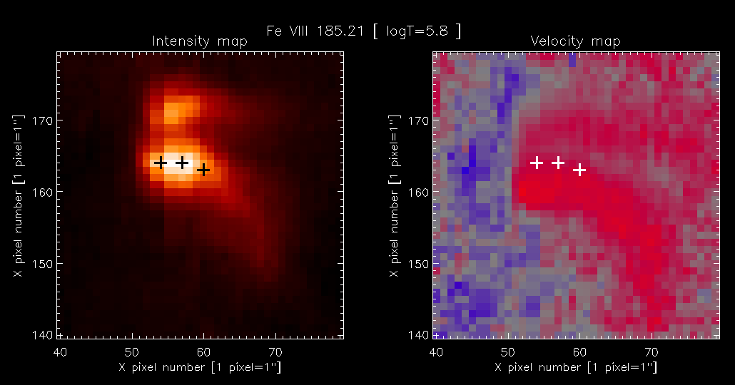
The velocity map shows structures that clearly correspond to the intensity structures, suggesting the loop footpoints are redshifted. Three crosses have been placed on the intensity map at where the intensity peaks in the Y-direction. It is seen, however, that the positions of the crosses on the velocity map do not correspond to where the redshift is largest.
While this may seem to be an interesting physics result, evidence from velocity maps of a range of different solar structures suggests that this intensity-velocity spatial offset is actually an instrumental effect. To state the effect simply:
"Wherever there is a decreasing intensity gradient from north to south, the centroid of the emission line will be artifically shifted to longer wavelengths (redshift); and wherever there is a increasing intensity gradient from north to south, the centroid of the emission line will be artifically shifted to shorter wavelengths (blueshift)."
A similar phenomenon was observed in SOHO/CDS data and was explained by Haugan (1999) as being due to an "elliptical, tilted point spread function". This is illustrated in the plot below.
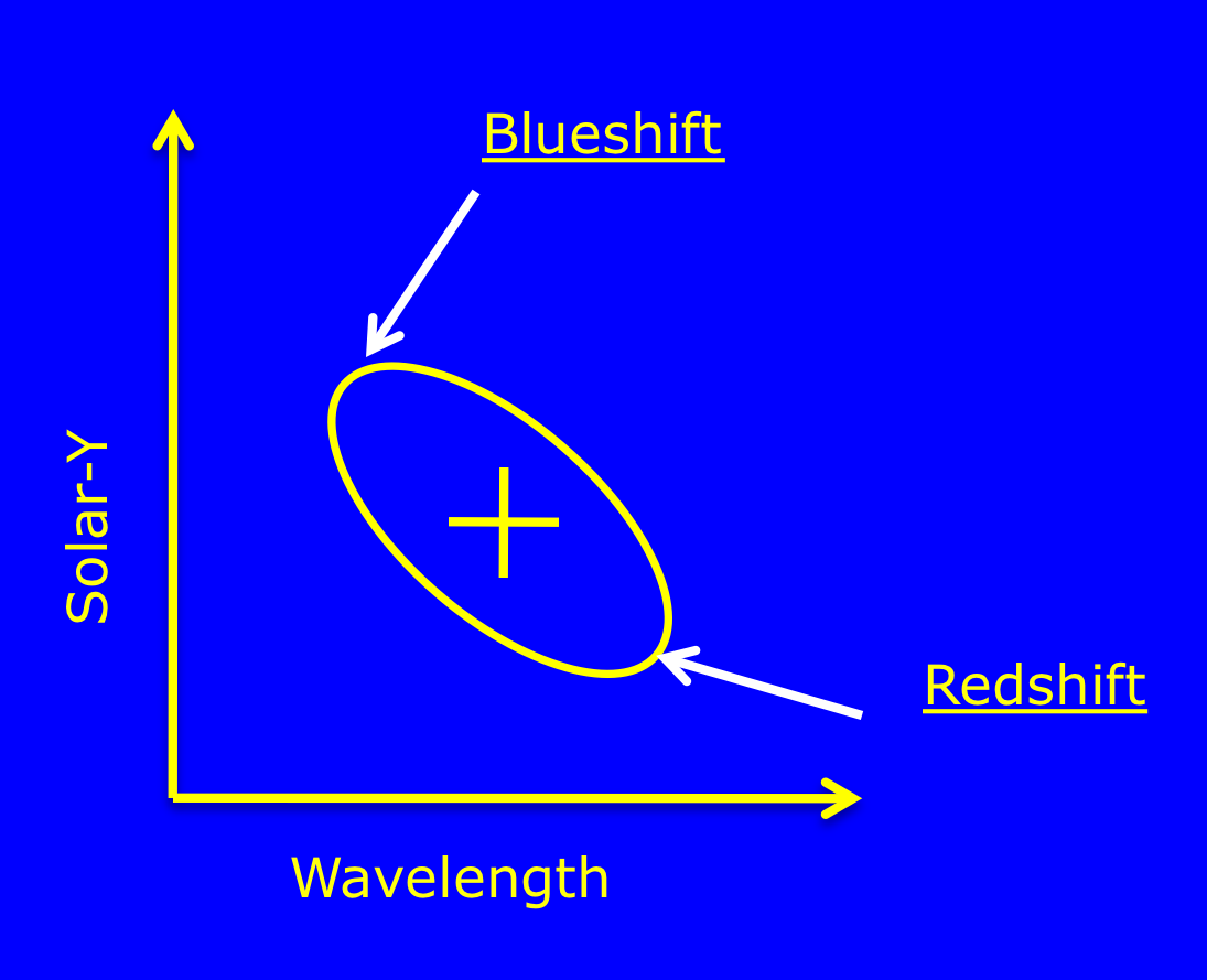
A point source imaged by EIS will yield an elliptical spot on the detector whose axes lie at an angle to the detector's axes. The spot will spread over a number of pixels on the detector and if Gaussian fits are performed at each pixel there will appear to be a blueshift on the north side of the spot and a redshift on the south side of the spot.
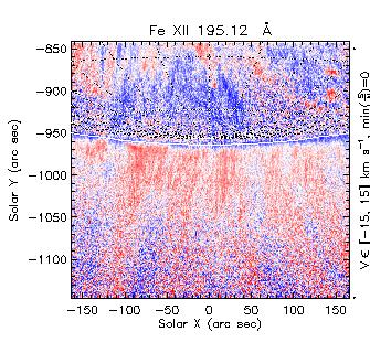
Tian et al. (2010) studied an EIS raster at the north coronal hole and they noted two features in the velocity maps that are likely due to the tilted point spread function. The Fe XII and Fe XIII velocity maps from their Figure 1 show distinctive ridges of redshift along the limb. For these coronal lines the region just above the limb is significantly more intense than the region just below the limb, and so there is a decreasing intensity gradient from north to south. From the statement above this means there is expected to be a redshift in this region, as observed.
The second feature noted by Tian et al. (2010) is that all the bright points found in the coronal hole have redshifts on one side and blueshifts on the other. Inspection of the images shows that the bright points are blueshifted on the north side and redshifted on the south side. This is again explained by the tilted point spread function.
If a velocity map is created at the south pole, then it is found that there is ridge of blueshift along the limb as shown in the thumbnail velocity map below, obtained from the Oslo Hinode Science Center.
