EIS Data Analysis Userguide

EIS Data Analysis Userguide

The analysis guide covers the basics of getting started with the data analysis. You can also find some tips as knowledge progresses on the EIS wiki /eiswiki/ which is our help desk.

Quick links:

How do I get my hands on the data?

What type of data is there?

How do I read and extract data?

How do I calibrate my data?

How do I display the data?

How do I do cosmic ray removal?

How do I calculate velocities, line widths etc.?

How do I identify lines in the spectrum?

How do I produce slot movies from rastered data?

How do I get my hands on the data

There are various means to do this:

The DARTS system at ISAS:

http://darts.isas.jaxa.jp/hinode/top.do

The ESA system in Norway:

http://sdc.uio.no/search/API12.php

The UK system at MSSL:

/SolarB/

Each of these systems has different ways of searching for data. The ESA one has thumbnails, the MSSL system has a movie maker and thumbnails for both level 0 data (unprocessed) and level 2 data (line shifts and line widths).

Finally you can use the eis_cat routine within IDL. This allows you to search for the data by remotely searching the EIS catalogue.

http://orpheus.nascom.nasa.gov/~zarro/idl/eis/eis.html

What type of data is there?

There are 3 different types of data files with EIS:

Level 0: these are reformatted data which are unprocessed. When you request data this is the data you normally get.

Level 1: We provide software for you to obtain level 1 data - this is the calibrated data. The routine is eis_prep.

Level 2: Level 2 data provides a quick look first cut at the velocities. Since this is an automated process it is not recommended that you use this for detailed scientific work, but merely as a quick-look to determine if there is anything interested in the data sets such as large velocities. You can obtained the level 2 data and have a look at it online. The level 2 data is produced only for 1" and 2" slit data.

How do I read and extract the data?

The easiest way of accessing data in a file called "mydatafile" is through the IDL procedure called eis_getdata:

IDL> eis_getdata, myfilename, wd, (iwin = iwin, /all, hdr = hdr, /ccsds)

The inputs parameters are:

myfilename: Name of data file (in CCSDS or FITS format. Default is FITS - see CCSDS keyword described below.)

The output parameters are:

wd: data cube returned. Could be called anything by the user.

The keyword parameters (optional) are:

iwin: Set this keyword to a series of line window numbers to return those line windows. e.g. iwin = [0,3,5] returns line wwindows 0, 3 and 5 from the raster.

all: set this keyword to return all line windows. If this is not set AND iwin is not set, line window 0 is returned as default.

hdr: Set this (e.g.hdr=hdr) to return the header information.

ccsds: Set this if the data file is a telemetry file (the default is FITS).

Example1: The data file myfilename is a FITS file containing a scanning raster with 200 raster positions, 512 pixels along the slit, 25 line windows each of 32 pixels width. Return line windows 3, 12 and 24. I also want the FITS header.

IDL>eis_getdata, myfilename, wd, iwin=[3,12,24], hdr = hdr.

The wd cube should now have dimensions: [32, 512, 200, 3] or [nlambda, nslit, nraster, nlines].

Example2: The data file myfilename is a `CCSDS file containing a full CCD exposure. 512 pixels along the slit, 4 line windows each of 1024 pixels width. Return all line windows. I also want the telemetry header

IDL>eis_getdata, myfilename, wd, /all, hdr = hdr, /ccsds

The wd cube should now have dimensions: [1024, 512, 1, 4] or [nlambda, nslit, nraster, nlines].

To return data from one spectral line you can use the routine:

IDL> d= eis_windata(file, [iwin,keywords])

For those of you comfortable with objects, an alternative method is:

To create an EIS object, use:

0. IDL> obj = obj_new ('eis_data', filename,datasource='fits')

0. Each EIS fits file can include maximum 25 line-windows, ie. window 0, 1, ...,24.

0. The following example shows data for the 6th window acquired from the data object

0. IDL> iwin=5

0. IDL> wd=data->getvar(iwin)

IDL> data->getwin, iwin, wd, pos

There are various ways using objects to probe information - e.g. to get the spectral window size. The spectral line-window data has the dimension of data[xsize, ysize, nexp], ie. [X-direction, Y-direction, exposures].

0. Each window may has different xsize, ysize - to get xsize, ysize and nexp, using:

IDL> xsize=obj->getxw( )

IDL> ysize=obj->getyw( )

IDL> nexp=obj->getnexp( )

There are many different methods to use - in order to search through these use:

IDL> data->display_methods

IDL> data->display_all

How do I calibrate the data?

The eis_prep routine should cater for most of your calibration needs. You will need to setup setssw cds eis in order to run the cosmic ray removal routine. The routine eis_prep corrects for:

dark current subtraction

cosmic ray removal

flat field correction

hot pixels

absolute calibration

bad/missing pixels marked throughout

error saved in calibration object in eis_er_yymmdd_hhmmss.fits file

data contains pointer to calibration objects

object saved to file (level 1)

IDL>eis_prep,file,/def,/save

How do I display the data?

The EIS instrument is very flexible with many different modes available - hence there are different ways of looking at the data, some of which are described below. The main thing you need to consider is which slit/slot was used - 1", 2", 40" and 266".

(a) Showing spectrum data

When using the 1" or 2" slit rastering is often done. The dimension of raster scanning data is data[lambda, y, x]. If you do the following you can have a quick look at a movie of the spectrum.

IDL> window,0,xs=xsize[ iwin ],ys=ysize[ iwin ]

IDL> stepper,data

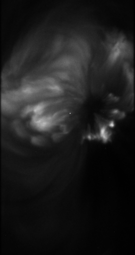
(b) Display slot picture

In case of the data was in the slot mode (i.e. 40" or 266"), then the following will display the data. To show slot picture in correct direction, it is necessary to reverse left-right (ie. east-west) direction.

IDL> window,0,xs=xsize[ iwin ],ys=ysize[ iwin ]

IDL> tvscl,rotate (data[ *, *, 0 ], 5 )

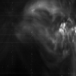
(c) Displaying raster data

For raster scanning data, integrating the spectrum along wavelength direction gives the image of a particular spectral band.

IDL> intensity = rotate (total (data, 1), 1)

IDL> window,0,xs=nexp,ys=ysize[ iwin ]

IDL> tvscl,intensity

How do I do Cosmic Ray Removal

Cosmic ray removal is included within eis_prep, but you may want to do this separately. There is a routine called "eis_despike.pro" to do cosmic ray removal for one line window and on exposure. So far there is now script available to process many line windows and several exposures automatically. eis_despike is based on the SSW procedure called "new_spike.pro", which has been extensively used and tested on CDS data.

To do cosmic ray removal do:

SSWIDL> eis_despike, wd_in, wd_despike

INPUT:

wd_in: Linw window before CR removal

OUTPUT:

wd_despike: Line window after CR removal

KEYWORDS:

no_neighbours

no_fill

info

For description of keywords, see documentation of new_spike.pro in SSW.

I want to calculate velocities, widths etc. How?

There are two ways of calculating intensity, velocity and width from the line profiles. It can either be done from the QL control window XCONTROL, by clicking the "moments" button, or it can be done using a procedure called "eis_getmoments". In the first case, results are displayed using the QL, in the latter, the user will get hands on access to the calculated quantities.

In both cases, the user need to manually interact in order to define line and continuum pixels. In the future this could be done automatically from e.g. line IDs, but so far the logic around this has not been worked out. Input from the planning tool may be needed, and we're not there yet.

The usage of eis_getmoments is decribed in what follows:

IDL> eis_getmoments, file, int, vel, wid, iwin =iwin, all = all, gauss = gauss, $ moment = moment, ccsds = ccsds, lamtype = lamtype, $ line_def = line_def

INPUTS

file: Name of file (string) containing EIS data (and headers).

KEYWORD PARAMETERS:

iwin: The line number indexes (starting with 0, max 24.)

all: process all line windows

gauss: set this to use gaussian fits to calculate int, vel, wid. This calls a CDS procedure called XCFIT.

moment: (Default) Use moments to calculate int, vel, wid

line_def: Use pre-stored pixel definitions for line and continuum. (not yet fully implemented!!) These are stored in text files, as pixels defining where on the CCD the spectral line and it's (to be subtracted) continuum is.

lamptype: Can take two values: lamtype='pix' (DEFAULT) for pixel wavelength scale or lamtype='wav' for wavelength scale in Ångstrøm.

ccsds: set this keyword if telemetry file. Standard is fits.

OUTPUTS:

int: intensity (0th order moment). Normally int[x,y, nwin]

vel: velocity (1st order momemt). Normally vel[x,y, nwin]

wid: width (2nd order moment). Normally wid[x,y, nwin]

example 1: Calculate int, vel wid, from Line window 0 from CCSDS file1= 'file1.dat':

IDL> eis_getmoments, file1, int,vel,wid, iwin=0, /ccsds

example 2: Get line windows 2 and 3 from fitsfile file2='file2.fits'. Use wavelength scale and gaussian fits:

IDL> eis_getmoments, file2,int,vel, wid, iwin=[2,3], lamtype='wav', /gauss

How do I identify lines in the spectrum?

You can look at the spectrum at each pixel location either within the quicklook software 'xfiles' or else you can use:

IDL>eis_raster_browser,file

If you want to then identify the lines you can make use of CHIANTI through:

IDL>xspecplot

Be warned that not all lines have yet been identified in the EIS wavebands so there is most likely some missing from CHIANTI!

I want to make a movie from several rasters. How?

This is an example of how you concatenate files using objects to create a movie.

We have dowloaded a number of files for Feb 19, 2007 to an appropriate directory

[elstar:2007/02/19] viggoh% ls eis_l0_2007*.gz

eis_l0_20070219_112228.fits.gz eis_l0_20070219_140814.fits.gz eis_l0_20070219_150131.fits.gz

eis_l0_20070219_134135.fits.gz eis_l0_20070219_143452.fits.gz eis_l0_20070219_193631.fits.gz

and we happen to know (we looked using the SSW QL `xfiles’ routine) that it is the files spanning 13:41 to 15:01 that interest us. Before concatenation and analysis we will prep them to remove dark current, cosmic rays, hot pixels and convert to physical intensity units as well as calculate the measurement error. All of this is done by the SSW routine eis_prep.

IDL> f0=file_search('eis_l0*.gz')

IDL> f0=f0[1:4]

IDL> print,f0

eis_l0_20070219_134135.fits.gz eis_l0_20070219_140814.fits.gz eis_l0_20070219_143452.fits.gz

eis_l0_20070219_150131.fits.gz

IDL> for i=0,n_elements(f0)-1 do begin eis_prep,f0[i],/def,/save

This is the default method of calling eis_prep; /def means that default methods for cleaning up the data will be used, /save means that the prepped data will be saved in an `eis_l1’ fits file while the error estimate will be saved in an `eis_er’ fits file.

Concatenation

Observations are often spread over several fits files, when analysing these it will often be advantageous to concatenate. Here we will put all the slot observations of the Fe XII 195 line into one cube.

IDL> f1=file_search('eis_l1*.fits')

IDL> f1=f1[1:4]

IDL> print,f1

eis_l1_20070219_134135.fits eis_l1_20070219_140814.fits eis_l1_20070219_143452.fits eis_l1_20070219_150131.fits

IDL> concat_cube,f1,4,cube,time_cube,line_id=line_id