This is EIS Discussion Area page.
#
Changes to eis_wave_corr and eis_getwindata: September 27, 2010.#
The functionality of eis_wave_corr has been changed. It now calls the procedure eis_wave_corr_hk to compute the time-dependent wavelength correction. This routine is based on the algorithm produced by Kamio-san. It is possible to use the "old" method by using the the "old" keyword. Note that eis_wave_corr_hk requires housekeeping files to work.
The functionality of eis_getwindata has also been changed. The default behavior is to calculate the wavelength correction for the data window and include this information in the structure. The use of the keyword "no_wave_corr" causes the wavelength correction not to be calculated, but arrays are allocated for later use.
A Comment on Using Fe XII 195 for Studying Nonthermal Widths and Doppler Shifts#
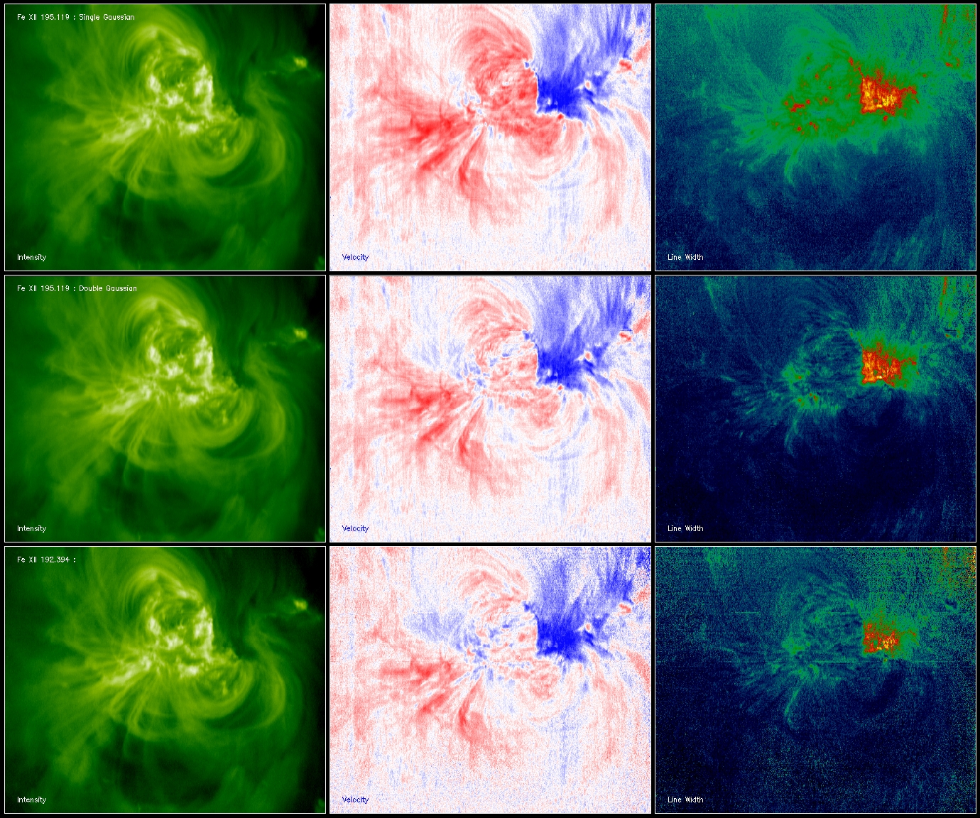
Fe XII 195 is a core line and is present in almost every EIS study. It has been noted, however, that there is a subtle contribution of Fe XII 195.18 to the wing of the observed line profile. This component is density sensitive and can make an important contribution to the line in active regions. The intensity of this component is generally very small (<15% of the total), it does, however, alter the calculation of the line width and centroid. A two Gaussian fit can be performed on the observed line profile but it is necessary to constrain it. One scheme is to set the line widths of both components to be equal and to fix the difference between the two line centroids to be 0.06 Angstroms. This is not difficult to implement in MPFIT.
The following images illustrate the differences between a single Gaussian fit (top), a two Gaussian fit (middle), and a single Gaussian fit (bottom) to the Fe XII 192.394, which appears to be unblended. The single Gaussian fit suggests larger nonthermal widths and Doppler shifts in the active region than are seen in the two Gaussian fit or in the Fe XII 192.394 line.
 |
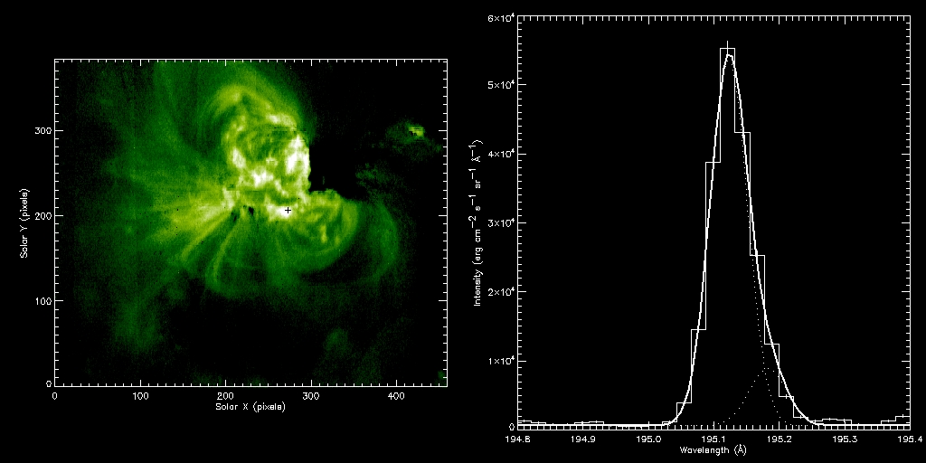
Here is an example profile fit. The image is the intensity in Fe XII 195.18.
 |
A detailed discussion on this can be found in the following paper by Peter Young. Also note that you can view higher resolution images by looking at the "Attach" tab.
A Comment on the Temperature of Formation for Fe VIII#
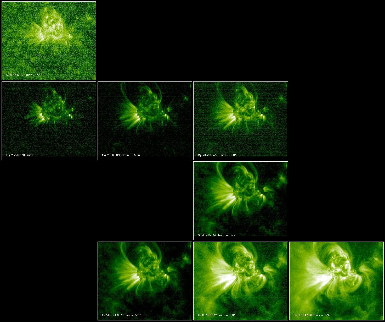
It has been noted that Fe VIII and Si VII rasters look nearly identical (Young et al. 2007) but the temperature of formation for the two ions are separated by about 0.2 dex. This image illustrates this by comparing Mg, Si, and Fe images in this temperature range. These data suggest that Fe VIII and perhaps Fe IX are formed at higher temperatures than suggested by the ionization balance calculations of Mazzotta et al. (1998).
 |
Note that you can view higher resolution images by looking at the “Attach” tab.
An explanation for this observation is given by Brooks, Warren, and Young (2011).
Deconvolving coronal features from the He II 256 blend#
He II 256.32 is a self-blend of two He II lines and is also blended with four coronal lines. This section provides some information for those hoping to accurately extract the He II component from the blend.
Missing exposures and bright exposures#
Since the change to S-band operations in 2008 it has been common to see missing exposures when forming rasters from EIS data. Another feature has been the appearance of anomalously bright exposures. The link below shows examples from one raster data-sets.
PRY_footpoints_HI2 raster on, 11-Dec-2009, 19:50