He II 256 in off-limb quiet Sun spectra#
Since the cool He II 256 will become weak in off-limb spectra then this is a good place to study the contributions of the blending coronal lines.
According to CHIANTI the wavelengths of the various lines are:
He II 256.317
He II 256.318
Si X 256.366
Fe X 256.398
Fe XII 256.410
Fe XIII 256.422
The first thing to note is that the four coronal lines all lie on the long wavelength side of the He II lines. The two He II lines themselves can effectively be treated as a single line.
The off-limb spectrum being used is from 2007 March 9 20:03. Using the procedure outlined elsewhere on the wiki a spatial region has been averaged to produce a single spectrum from which emission lines can be measured. Using standard density diagnostics we find the density is about 10^8.5.
Fit to 256 feature#
In the off-limb spectra, the feature at 256.3 is seen to comprise of two components that can be fit with two Gaussians. I find fit parameters of
256.321 0.071 37.1
256.413 0.106 139.2
(centroid, width and intensity, respectively). Based on the wavelengths above it seems, to first approximation, that the long wavelength Gaussian represents the coronal lines, and the short wavelength Gaussian the He II lines. Below we check the combined intensity of the four coronal lines.
Si X 256.366#
This is the easiest line to deal with and is also the strongest of the four lines in the off-limb spectrum. 256.4 is related to the nearby 261.0 line by a branching ratio which means that the two lines have a fixed ratio in all conditions: 256.4/261.0 should be 1.12.
The intensity of 261.0 is found to be 84.3, implying the intensity of 256.4 is 94.7.
Fe X 256.398#
This transition is one of a number of 2P - 4D transitions in this part of the spectrum. By far the strongest is the Fe X self-blend at 257.26. Two further lines are at 266.1 and 255.4. Firstly it is interesting to check whether the unblended lines actually agree with each other. The measured intensities are:
Fe X 257.296 122.8
Fe X 266.122 3.3
Fe X 255.462 2.4
The 257 self-blend is density sensitive relative to the other two lines and between 10^8 and 10^9, the 266/257 ratio is about 0.025, and 255/257 is about 0.019. The measured ratios are 0.025 and 0.014. This agreement is reasonable and suggests that CHIANTI is doing a good job of predicting the strength of the 2P - 4D transtions.
Going back to the Fe X 256 line, CHIANTI predicts the 256/257 ratio is about 0.085, giving a predicted intensity for the 256.4 line of 10.4.
Fe XII 256.410#
The Fe XII 256 line is a 2D - 4F transition, and there are two other nearby lines from this multiplet that are relatively insensitive to the 256 line. However both lines are blended so it takes a little work to estimate the 256 contribution.
The two lines are measured to be
S X + Fe XII 259.527 56.0
Fe XII + Fe XIII 260.007 9.3
The first line is blended with the much stronger S X line. This can easily be accounted for by noting that the S X 259.5/264.2 ratio is predicted by CHIANTI to be almost constant with a value of 0.688, implying Fe XII has an intensity of 6.5.
Estimating the Fe XIII contribution to 260.0 is more tricky. The Fe XIII 251.9/260.0 ratio is density sensitive, but between 10^8 and 10^9 it is not so sensitive with a value of around 47. This implies Fe XIII makes a contribution of 1.5 to the blend at 260.0, leaving 7.8 for Fe XII.
CHIANTI predicts that Fe XII 260.0/259.5 should be 0.75, yet the above numbers give 1.2, so there's a significant discrepancy here.
Now CHIANTI predicts that Fe XII 256.4/259.5 should be about 2.7, and 256.4/260.0 should be about 3.5. This means that the Fe XII 256.4 will be somewhere between 17.6 and 27.3 depending on which ratio is used.
Fe XIII 256.422#
This line can be estimated by making use of the stronger Fe XIII line at 251.96, however 256.42/251.96 is density sensitive. For the off-limb spectrum we know the density is low, and the 256.42/251.96 is actually relatively insensitive to density over 10^8 to 10^9, with a value of about 0.17. The 251.96 measured intensity is 69.0, and the so predicted 256.42 intensity is 11.7.
Summary#
Combining the four estimated intensities gives a total of either 134.4 or 144.1, depending on which estimate of the Fe XII line intensity is used. These values are actually in very good agreement with the strength of the long wavelength Gaussian in the fit to the 256.3 feature mentioned above. This suggests that the method outlined above for estimating the intensities of the coronal lines actually works quite well.
Caveat In estimating the intensities above, it was necessary to assume a low density of < 10^9 in order to apply some of the ratios. In particular, this was necessary for Fe X, XII and XIII. This method would need to be revised for, e.g., an active region observation.
Variation of He II 256 profile across the limb#
To further investigate the He II 256 line, a large raster obtained at the limb has been studied to see how the line profile varies crossing from the disk to the limb.
The raster was obtained on 2007 December 12 at 10:42 (cam_ar_limb) and uses the 2" slit to raster an area of 360" x 512". The observation covers a large active region, but the bottom of the raster covers a relatively quiet region.
He II 256 spectra were generated for 25 positions by averaging Y-pixels 5 to 40 for 25 X-pixels spaced at 7 pixel intervals, beginning with pixel 2 which is inside the limb. I.e., the X-pixels used were 2, 9, 16, 23, etc., up to 170. The spectra were creating using the routine eis_mask_spectrum by creating pixel masks for each position.
The 25 spectra that resulted are plotted in the image below. The limb is found at about X=860. The Y-axis is intensity in erg/cm2/s/sr/angstrom, the X-axis gives the wavelength in angstroms but with 256 angstroms subtracted in order to make the plots easier to read.
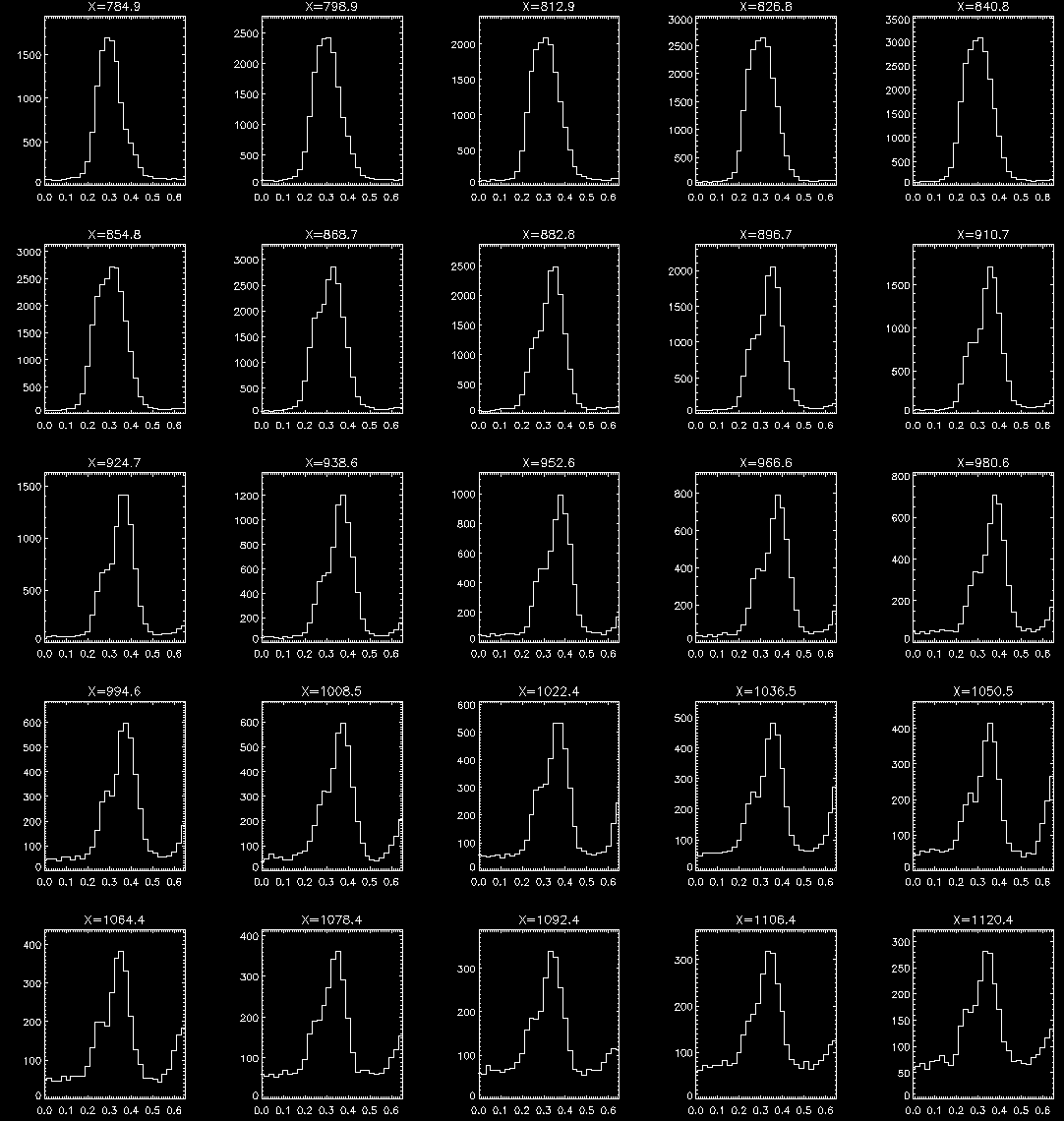 |
If we assume the He II component is on the short wavelength side, then we see it becoming weaker at X=868, which is just above the limb. By X=910 the short wavelength component is about a factor 2 smaller than the long wavelength component which we assume is the blend of the coronal lines. However, as X increases the short wavelength component remains approximately constant relative to the long wavelength component. Both components fall off in intensity with height
This behavior is not consistent with He II which we expect to drop sharply above the limb, but then remain approximately constant in intensity beyond a certain height due to the scattered light contribution. Instead it actually seems to behave like a coronal line.
The conclusion from this is that there is likely a coronal line at the wavelength of the He II 256.32 line and this is revealed when we cross the limb. Possibly this line could be one of the Si X, Fe X, Fe XII or Fe XIII lines discussed earlier if one of the lines has an incorrect wavelength. Alternatively it could be a previously unknown transition.