Spatial offset of velocity features relative to intensity features#
A striking feature of velocity maps obtained from EIS is that regions of strongest redshift or blueshift are often spatially offset from regions with the highest intensity. This is illustrated in the example below showing a pair of coronal loop footpoints observed in the Fe VIII 185.21 line.
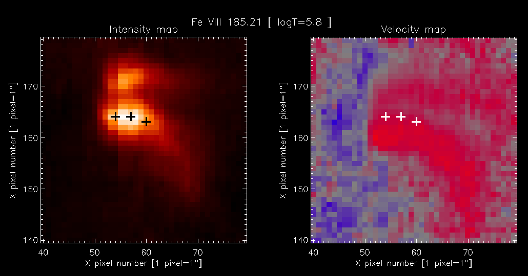 |
The velocity map shows structures that clearly correspond to the intensity structures, suggesting the loop footpoints are redshifted. Three crosses have been placed on the intensity map at where the intensity peaks in the Y-direction. It is seen, however, that the positions of the crosses on the velocity map do not correspond to where the redshift is largest.
While this may seem to be an interesting physics result, evidence from velocity maps of a range of different solar structures suggests that this intensity-velocity spatial offset is actually an instrumental effect. To state the effect simply:
"Wherever there is a decreasing intensity gradient from north to south, the centroid of the emission line will be artifically shifted to longer wavelengths (redshift); and wherever there is an increasing intensity gradient from north to south, the centroid of the emission line will be artifically shifted to shorter wavelengths (blueshift)."
The effect as shown in this loop feature was presented and discussed in Young et al. (2012) .
.
A similar phenomenon was observed in SOHO/CDS data and was explained by Haugan (1999) as being due to an "elliptical, tilted point spread function (PSF)". This is illustrated in the plot below.
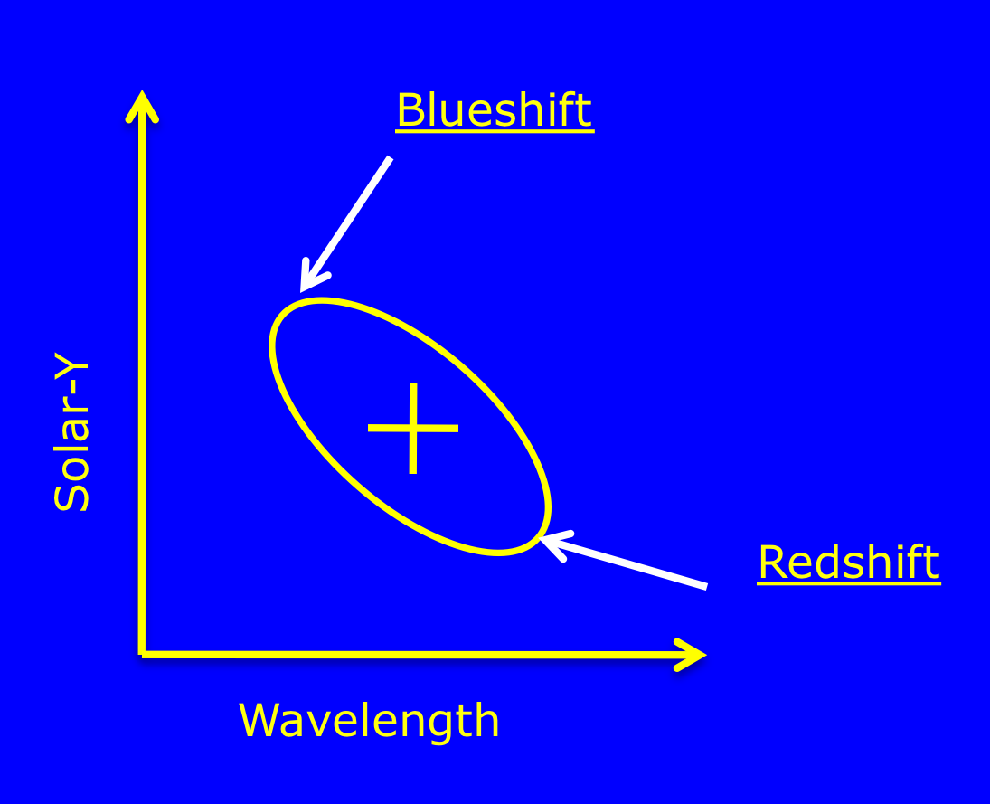 |
Such a PSF will yield an elliptical spot on the detector whose axes lie at an angle to the detector's axes. The spot will spread over a number of pixels on the detector and if Gaussian fits are performed at each pixel there will appear to be a blueshift on the north side of the spot and a redshift on the south side of the spot.
It is not clear yet if the EIS PSF has a tilted, ellipsoid shape like this but the velocity patterns observed suggest that it is similar. The shape would be expected to change along the slit and the thus the velocity patterns may vary with position within a raster.
Tian et al. (2010) studied an EIS raster at the north coronal hole and they noted two features in the velocity maps that can be explained by the tilted PSF model. The Fe XII and Fe XIII velocity maps from their Figure 1 show distinctive ridges of redshift along the limb. For these coronal lines the region just above the limb is significantly more intense than the region just below the limb, and so there is a decreasing intensity gradient from north to south. From the statement above this means there is expected to be a redshift in this region, as observed.
The second feature noted by Tian et al. (2010) is that all the bright points found in the coronal hole have redshifts on one side and blueshifts on the other. Inspection of the images shows that the bright points are blueshifted on the north side and redshifted on the south side. This can again be explained by a tilted PSF.
If a velocity map is created at the south pole, then it is found that there is ridge of blueshift along the limb as shown in the thumbnail velocity map below, obtained from the Oslo Hinode Science Center. This is consistent with a tilted PSF.
eis_l0_20070319_113354_6_0_vel.jpg
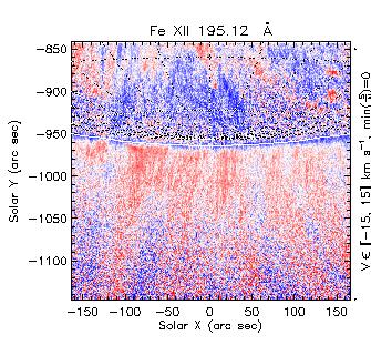
A key point to note is that a tilted PSF only affects features with significant intensity gradients, thus the main result of Tian et al. (2010) - the measurement of blueshifts in a large area of largely uniform intensity coronal hole - is not affected.
There is currently no software or prescription available to correct velocity maps for a tilted PSF. The following is a general observation:
The velocity shifts due to the PSF are around the 5 km/s level. I.e., if a velocity of V km/s is measured at the intensity peak (along the Y-direction), then a velocity of up to V+5 km/s will be measured to the south of the brightening, and a velocity of up to V-5 km/s will be measured to the north of the brightening. These shifts occur at about 3-4 pixels away from the intensity peak (see the footpoint image earlier in this document).
In general users should be cautious about showing velocity maps in publications, as a reader's eye tends to be drawn to the features that are most redshifted or most blueshifted. These features could be artificially enhanced by a tilted PSF and give a misleading impression of the velocity field of the structure.
When deriving velocities, the values obtained where the intensity peaks (in the case of bright points), or where the intensity is fairly uniform should be correct. In particular, velocity results such as the outflows detected in active regions (Harra et al. 2008, Doschek et al. 2008) will not be affected.
The EIS team is investigating the PSF function and whether this is responsible for the observed effect. Users are encouraged to look for the effect in their data and report their findings to their EIS team.
Update: There is now a Software Note 8 that describes this effect. Also, Warren et al. (2017) show in their Appendix that the velocity pattern observed in a flare current sheet, a bright elongated structure with strong gradients perpendicular to its axis, is consistent with the effect of an inclined PSF.