X-ray bright points (hereafter XBPs) are composed of small compact loops and are an ideal target
to study with current instrumentation due to their compact size (average value of 30'') and short lifetimes (average of 8 hours - see
Golub et al. 1974).
The Hinode satellite is especially suited to study small features like XBPs as it can utilise all three instruments to work together
and follow the entire evolution of a bright point from emergence to decay. Such a complete study is not possible for active regions
as they tend to last much longer often, out of view over the solar limb. The EUV Imaging Spectrometer (EIS), in particular, is great
for studying XBPs as they can easily be captured by the 1'' or 2'' slit with minimal exposures being needed to cover their area.
This means less 'temporal smearing' due to the rastering process, making more accurate analysis possible.
In
Alexander et al. 2011 we present a case study of a clear example of a XBP formed over a region of cancelling magnetic flux.
We have used all three instruments onboard Hinode to follow its evolution and measure as many plasma parameters as we can over the course of its lifetime.
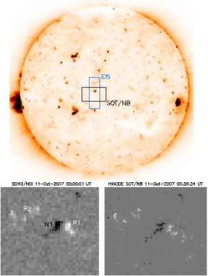
Figure 1 shows the location of our bright point on the solar disc. It had an average size of 15'' and a lifetime of around 12 hours.
The lower panels in
figure 1 show the location of the bright point seen by SOHO/MDI (left) and Hinode/SOT (right) - the stark difference in
resolution is clearly seen. The bright point is composed mainly of the areas labelled N1 and P1 but also included the second area of positive
flux labelled P2 which creates a secondary, weaker, loops system off to the east of the main bright point.
Figure 1:
The top panel shows a negative image of full-disc XRT Al_Poly/Open filter showing the location of the XBP and the FOV's of the EIS and SOT instruments.
The lower left panel shows SOHO/MDI data with the three main magnetic sources labelled. The lower right panel shows same-time SOT/NB data. The FOV of
both lower images is 100'' x 85'' » Click figure to see full-size image.
The Solar Optical Telescope (SOT) was used to study the evolution of these magnetic fragments and it can clearly be seen in
Figure 2 that this is a cancelling magnetic feature.
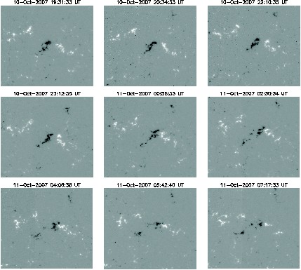
Figure 2: Hinode SOT NB FG Stokes V images of the bright point showing the merging and cancelling of the main positive
and negative areas of magnetic flux. The FOV is 80'' x 70'' and the range of the data is ±350 Gauss (click here for a movie of this
cancellation http://www.star.uclan.ac.uk/~cea/movies/xbp_sot_cea_movie.mov)
Using these SOT observations, we were also able to extrapolate the potential magnetic field structure and compare this to what we see in the X-ray
images.
Figure 3 shows two examples of this comparison and it can be seen that the potential field extrapolations were a good visual
fit to the observed coronal loops meaning that the magnetic field was not too far from a potential state (see
Alexander et al. 2011 for details and
Perez-Suarez et al. 2008
for similar results).

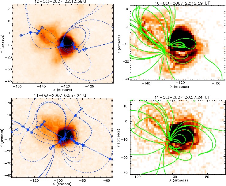
Figure 3:
Figure showing two examples of our comparison between the X-ray
emission seen in XRT and the similarities to the potential field
model applied. The two figures on the left show negative XRT images overlaid
with the photospheric footprints of the calculated topological
structure of the extrapolated magnetic field. Positive magnetic sources
are labelled as ⊕, negative magnetic sources as ⊗,
positive null points as ∇, negative null points as
Δ, spines as solid curves, and the intersections of
separatrix surfaces with the photosphere as dashed curves. It is
possible to form a good impression of the whole 3D magnetic field
structure, given that each null point's associated 3D separatrix
surface must close via spine field-lines in the photosphere in cases
where its own two separatrix traces do not terminate at the same
source. No field-line can cross a separatrix surface or a spine. The
two figures on the left show the same XRT images after being put
through an edge-detection process. These images have then been
overlaid with field-lines (in green) generated by the potential field
model to identify any structural similarities. » Click figure to see full-size image.
Using the available 22 EIS rasters (taken 30 minutes apart) we were able to study some important plasma parameters of the XBP.
We used the line ratio method using Fe XII lines to measure how the density changed over time and found it to have an average
value of 4.95 x 109 cm
-3, which declined by around 40% as the cancellation progressed. The EM loci method was also used with
EIS data to infer a steady temperature of log Te [K] ~ 6.1.
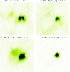
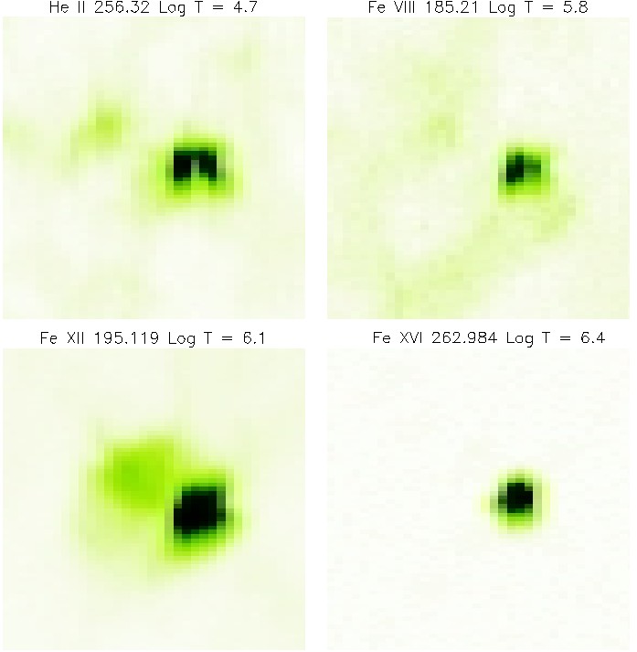
Figure 4 shows four examples of EIS intensity maps of the XBP at different temperatures. The top left panel shows a
chromospheric He II line which shows the lower structure of the XBP and exhibits a bipolar structure in the main body of the bright point which
we interpret as the footpoint locations of the (unresolved) system of hot loops. The lower left panel shows emission in the Fe XII 195 line and
clearly shows the main structure of the bright point alongside the secondary loops mentioned above.
Figure 4:
Negative EIS intensity maps of the XBP in different spectral lines on 11-Oct-2007 at 00.10.47 UT. The FOV is 70'' x 70'' » Click figure to see full-size image.
Plasma flows were studied using the strong line Fe XII 195 after correcting for the orbital variation of the wavelength
scale (see
Del Zanna, 2008a).
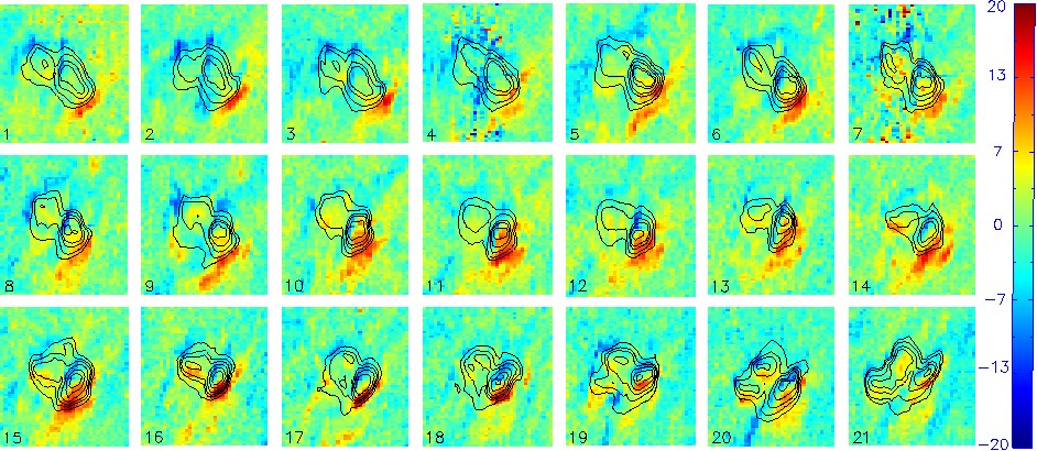
Figure 5 shows a time series of Dopplergrams of the area over the XBP over 12 hours at 30
minute intervals. It can be seen that even on the relatively short timescale of 30 minutes, changes are observed in the
strength and structure of the velocity flows suggesting that these flows are occurring on timescales smaller than the observations we have.
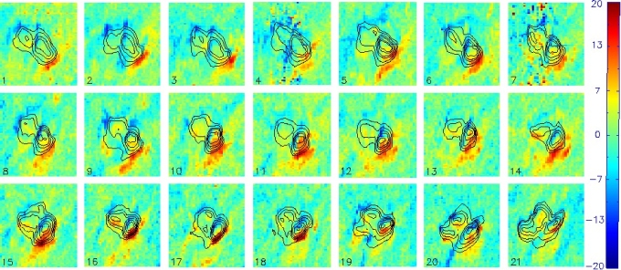
Figure 5:
Sequence of Dopplergrams of area around XBP from 18:45 on the 10-October-2007 every 30 mins until 06:32 on 11-Oct-2007. Velocities shown are
between ± 20km/s and are over-plotted with intensity contours. The FOV of each box is 70'' x 70''. » Click figure to see full-size image.
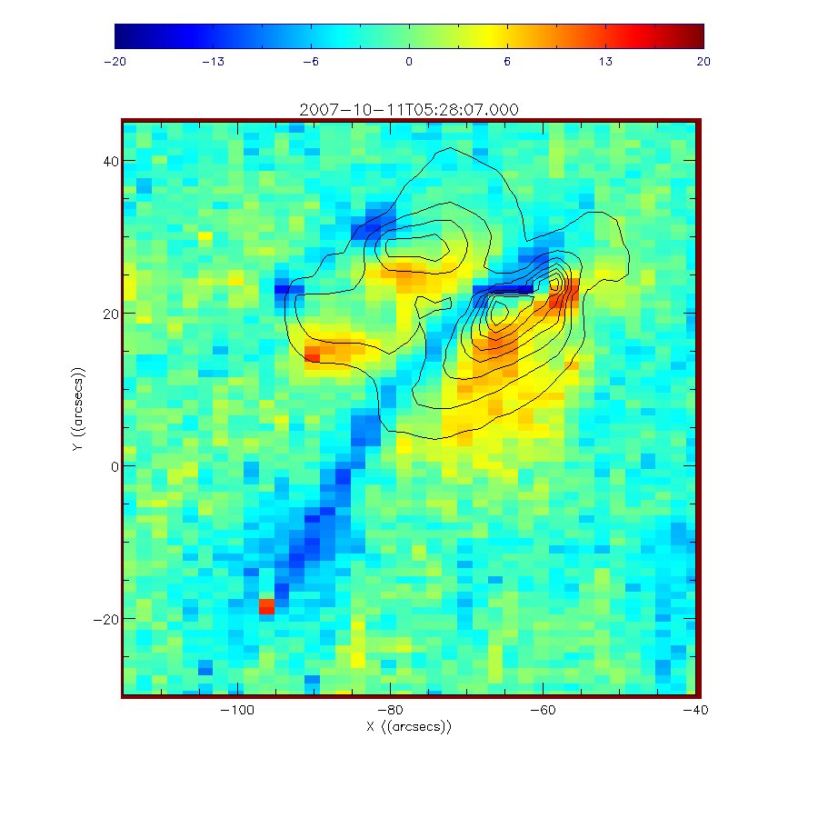
There is a persistent blueshift in the area between the main bright point and the secondary loop system. This is most clearly seen in
Figure 6 which
shows the 20th frame of
Figure 5 more clearly. This image shows a clear set of redshift-blueshift pairs on either side of each intensity contour peak
as well as a very strong blueshifted strip between the two loop systems.

Figure 6: Dopplergram of XBP at 05:28:07 UT on the 11-Oct_2007 with intensity contours overplotted. » Click figure to see full-size image.
The Dopplergrams clearly indicate a variable pattern which is somewhat puzzling, considering that the overall intensity pattern does not change so rapidly. Similar
patterns of red and blue-shifts were found in active regions (see e.g.
Del Zanna 2008b), but they were stationary over long times. It is quite possible that the
Doppler-motions are related to chromospheric evaporation (blue-shifts) and subsequent draining (red-shifts) following cooling. However,
Brosius et al. 2007 suggested
the possibility that, if outflows are connected to chromospheric evaporation, they would likely decrease in time, something that we do not see. Higher cadence
observations with EIS will better reveal the pattern and links between what we see in the magnetic structure on the photosphere and the corresponding changes
in the plasma velocities observed in the corona.
References:
Alexander, C. E., Del Zanna, G., & Maclean, R. C. 2011, A&A, 526, 134
Brosius, J. W., Rabin, D. M., & Thomas, R. J. 2007, ApJ, 656, L41
Del Zanna, G. 2008a, A&A, 481, L69
Del Zanna, G. 2008b, A&A, 481, L49
Golub, L., Krieger, A. S., Silk, J. K., Timothy, A. F., & Vaiana, G. S. 1974, ApJ, 189, L93
Perez-Suarez, D., Maclean, R. C., Doyle, J. G., & Madjarska, M. S. 2008, A&A, 492, 575