Hinode/EIS Measurements of Active Region Magnetic Fields
E. Landi (University of Michigan), R. Hutton (Fudan University), T. Brage (Lund University), W. Li (Lund University)

The magnetic field of the solar corona is one of the most critical parameters in solar physics, as it lies at the core of the physics of the solar corona and of the interactions between the Sun and its planetary system. The coronal magnetic field has proved very elusive to infer directly. Indirect measurements have been carried out studying long-duration coronographic observations of coronal waves from CoMP (Yang et al. 2020), but only at the limb, and coronal loop seismology (De Moortel et al. 2016). Spectropolarimetric measurements suffer from a few limitations, such as their being limited to the limb, and the weakness of some spectropolarimetric signatures themselves. The only disk measurements come from radio observations, which provide the magnetic field at different heights within the same structure, but not the actual height of the structure itself.
Recently, Li et al. (2015, 2016) and Si et al. (2020a) reported on a Fe X atomic structure property which makes the wavefunction composition of the 3s23p43d4D7/2 atomic level of Fe X sensitive to the presence of an external magnetic field, by mixing it with the nearby 3s23p43d4D5/2 level. This mixing induces a new Magnetically Induced Transition (MIT), which connects the 4D7/2 to the ground level in addition to the M2 existing transition, with an Einstein coefficient whose value depends on the magnetic field strength B (Figure 1). To a first approximation, the transition probability of the MIT transition depends on B2:
AMIT ∝ AE1 [B2 / (ΔE)2],
where AE1 is the Einstein coefficient of the E1 transition connecting the 4D7/2 level to the ground, and is the energy difference between the 4D5/2,7/2 levels. As shown by Li et al. (2015), the accidental pseudo-degeneracy of these two levels in Fe X causes this MIT to be sensitive to fairly small magnetic fields. The E1 and M2 transitions from the 4D5/2,7/2 levels result in the Fe X 257.26 Å line, one of the brightest in the Fe X spectrum, routinely observed by the EIS spectrometer from the start of its mission: the MIT transition can thus in principle be used to measure the magnetic field anywhere in the solar corona from 2007 onward.
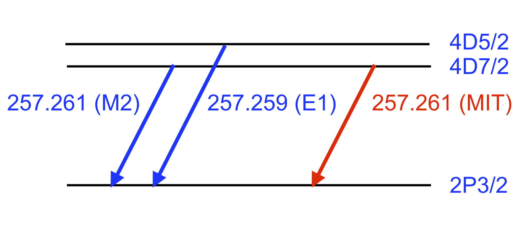
Figure 1:Fe X atomic levels involved in the MIT diagnostic technique.
Any Fe X line intensity ratio involving the 257.26 Å is dependent on the magnetic field. The best ratio in the EIS wavelength range is the one with the 184.54 Å line, due to its brightness and position in the EIS detector.
There are two important features that need to be considered:
A. the upper 4D7/2 level is metastable, so that all ratios involving the M2 and MIT lines are density sensitive; and
B. the EIS 257.26 Å is an unresolved blend of the E1, M2 and MIT transitions.
The first property requires knowledge of the electron density Ne before determining B. The second property forces us to determine the MIT and M2 individual intensities by intensity ratios. Also, the magnetically insensitive E1 transition dominates the blend as collisions with free electrons de-populate the 4D7/2 level and decrease the intensity of the M2 and MIT lines, and limits the sensitivity to the magnetic field of any ratio involving the 257.26 Å line.
There are three methods to measure the coronal magnetic field using the 257.26 Å line.
Direct technique: Calculate the intensity ratio of the entire (E1+M2+MIT) blend with another bright Fe X line as a function of B after Ne has been measured, and compare it with observations. Si et al. (2020b) used the 174.53/257.26 intensity ratio. The main limitation of this method is its limited sensitivity.
Weak field technique: If B < 150-200 G, the MIT transition is weaker than the M2 one and does not affect the 4D7/2 level population, so that the Fe X intensity ratios involving the M2 transition do not depend on B. This allows us to subtract the cumulative (E1+M2) contribution (calculated with CHIANTI) from the observed intensity, directly yielding the MIT intensity. This allows us to determine the MIT/M2 branching ratio as
[IMIT/IM2] = [I257/I184] R[184 / M2] - R[(E1 + M2) / M2]
where the R ratios are calculated with CHIANTI, and I257 and I184 are the observed EIS intensities. The dependence of the branching ratio on B is shown in Figure 2 (left). Ne limits the minimum B strength that can be measured to ∼50 G in active regions, and ∼10-20 G in the quiet Sun where density is lower.
Strong field technique: When B > 150-200 G, the M2 intensity depends on B, and the weak-field technique can not be used. As the E1 transition is still independent of B it can be subtracted from the 257.26 Å line, and the intensity ratio
[(IMIT + IM2) / I184] = [I257/I184] - R[E1 / 184]
can be calculated with CHIANTI (as shown in Figure 2 right). This ratio is less sensitive to B than the branching ratio technique, but is still an improvement over the direct technique.
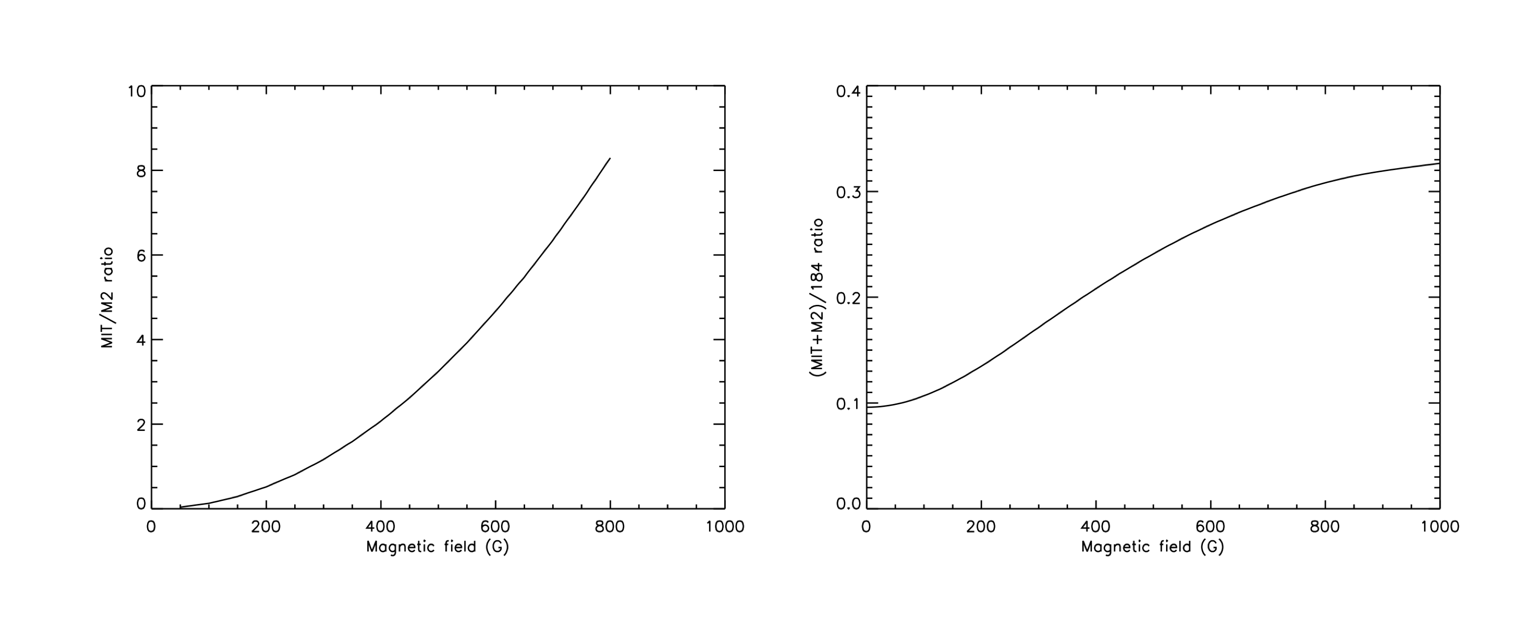
Figure 2: AMIT/AM2 branching ratio as a function of magnetic field strength (in G). Right: Example of the strong-field diagnostic technique: ratio of (MIT + M2) line
intensities to the 184.52 Å line intensity calculated as a function of magnetic field strength (in G).
Examples of Application
The EIS data set has been routinely observing the necessary spectral lines to apply the above technique, by including the Fe X 257.26 Å and 184.54 Å lines, and line pairs to measure the electron density. Landi et al. (2020a) include a complete list of the 98 EIS observing sequences that include the lines necessary to apply this diagnostics.
We show an example of the application of this technique on EIS data in Figure 3, which displays observations of AR 10978 taken by EIS on 12-Dec-2007 (top), 15-Dec-2007 (middle), and 18-Dec-2007 as AR 10978 rotated from the disk to the limb. No spatial averaging was made. The left column shows the intensity of the 184.54 Å line, and the right column the resulting magnetic field diagnostics.
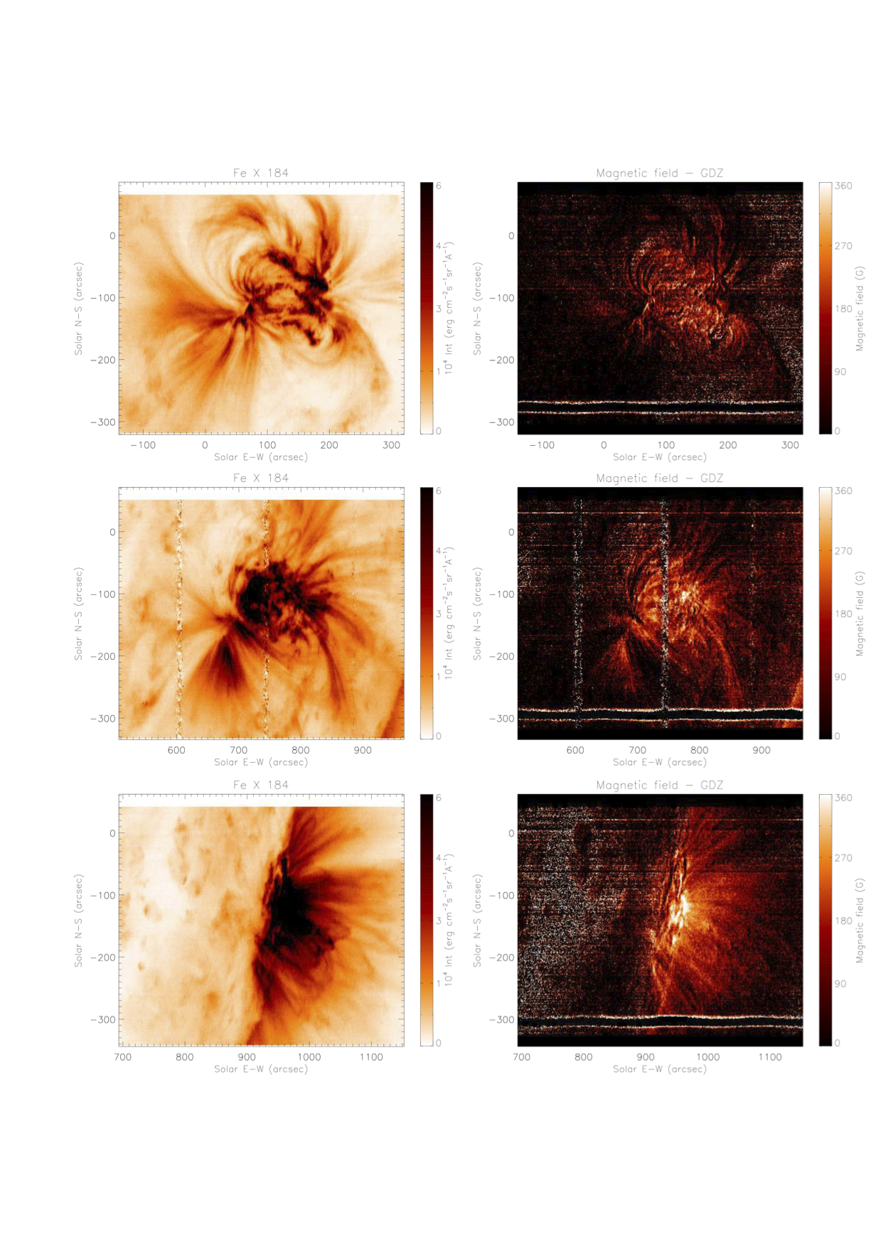
Figure 3: Maps of 184.54 Å line intensities (left column) and magnetic field strength (right column) for AR 10978 observed in December 2007 as it rotated on the disk. Top: 12 December 2007; Middle: 15 December 2007; Bottom: 18 December 2007.
This diagnostic technique measures the magnetic field strength, not its direction. However, the brightness of the Fe X lines involved allows to associate B values to individual loop structures provided they are resolved in the EIS intensity image itself. Furthermore, high cadence observations can help determine the temporal evolution of the magnetic field, a critical factor in the buildup of flares and CME eruptions.
Limitations and further work
There are a few limitations in the present technique:
1. The most important limitation lies in the EIS intensity calibration, as the 257.26 Å line lies in the LW channel, all other bright Fe X lines lie in the SW channel. The relative SW-LW intensity calibration, still uncertain, is the single most important source of uncertainty in the present technique;
2. The MIT intensity depends on the value of energy difference between the 4D5/2,7/2 levels. This value is known with a 20% accuracy from recent SUMER measurements (Landi et al. 2020b) but improvements are needed;
3. This diagnostic technique depends on the accuracy of the atomic data used to calculate the necessary Fe X intensity ratios from CHIANTI. While current CHIANTI values seem to be reasonably accurate, new calculations with larger atomic models for the scattering problem are needed;
4. This technique is best suited for magnetic fields larger than ∼10 G (quiet Sun) and ∼50 G (active regions). While future developments may lower these limits, applications for quiet Sun and coronal hole magnetic fields are at the edge of the technique's sensitivity.
We strongly urge the EIS team to improve on the relative LW-SW intensity calibration to decrease the uncertainty in the measurements of B.
For more details, see Landi et al. (2020a), ApJ, in press:
Hinode/EIS measurements of active region magnetic fields
References
De Moortel, I., Pascoe, D.J., Wright, A.N., Hood, A. 2016, Pl. Phys. and Contr. Fusion, 58, 014001
Landi, E., Hutton, R., Brage, T., Li, W. 2020a, ApJ, in press
Landi, E., Hutton, R., Brage, T., Li, W. 2020b, ApJ, 902, 21
Li, W., Grumer, J., Yang, Y., et al. 2015, ApJ, 807, 69
Li, W., Yang, Y., Tu, B., et al., 2016, ApJ, 826, 219
Si, R., Li, W., Brage, T., Hutton, R., 2020a, J. Phys. B, 53, 095002
Si, R., Brage, T., Li, W., Grumer, J., Li, M., Hutton, R., 2020b, ApJ, ApJL, 898, L34
Yang, Z, Bethge, C., Tian, H. et al. 2020, Science, 369, 694
Next EIS Nugget »» coming soon...
TBC
Last Revised: 27-Oct-2011
Feedback and comments: webmaster
|