Comparisons of LOS Doppler velocity and non-thermal line widths in the off-limb solar corona measured simultaneously by CoMP and Hinode/EIS
Jae-Ok Lee - Korea Astronomy and Space Science Institute
It is generally believed that Alfvén waves in the solar corona are one of the main energy sources for coronal heating and solar wind acceleration. In order to find the Alfvén wave signatures in the off-limb solar corona, observations of the line of sight (LOS) Doppler velocity and non-thermal line width by Coronal Multichannel Polarimeter (CoMP, Tomczyk et al. 2008) and Hinode/EUV Imaging Spectrometer (EIS, Culhane et al. 2007) have been used. Here, the CoMP measures the linear polarization of the Fe XIII 10747 Å and 10798 Å coronal forbidden emission lines by using three-wavelength data with a low spectral resolution of 1.2 Å. The CoMP provides their peak intensity, LOS Doppler velocity, and line width simultaneously over a field of view (FOV) ranging from 1.05 to 1.40 R sun with high spatial resolution of 4.5″/pixel and temporal cadences of 30 seconds. On the other hand, the EIS measures high resolution spectra in two wavelength bands, 170-211 Å and 246-292 Å, with a high spectral resolution of 0.0223″/pixel and with different sizes of slits (1″ and 2″) and slots (40″ and 266″). The EIS provides the spectral line intensities, LOS Doppler velocities, and line widths simultaneously at specific slit positions up to 1.5 R sun.
As described above, since CoMP can provide 2-D Doppler velocity and non-thermal line maps for the off limb corona from 1.05 to 1.40 R sun every 30 seconds, it is suited to examine propagating coronal Alfvén wave signatures on different coronal regions at the same time, and estimate their origins, energy fluxes, and dissipations. However, it usually obtains the spectroscopic quantities using three-wavelength data at the Fe XIII lines with a low spectral resolution of 1.2 Å. This limitation is likely to affect the Doppler velocity and non-thermal line width measurements. For example, if the actual spectral line window including strong emission lines is broader than the observed line window (3.6 Å), the measured CoMP non-thermal line widths might be underestimated. If the actual spectral window is narrower than the spectral resolution (1.2 Å), the measured values might be overestimated. In this study, we examine whether the CoMP LOS Doppler velocity and non-thermal width obtained by using only the three-wavelength data are reliable or not. For this, we compare the two physical quantities measured simultaneously from CoMP Fe XIII 10747 Å lines and EIS Fe XII 195.12 Å lines for investigating flaring active region (AR11654 on 2013/01/20) and two quiescent active regions (AR 11461 and 12149 on 2012/04/16 and 2014/09/01). The EIS Fe XIII 202.04 Å lines are used for examining an equatorial quiet region on 2013/02/26, two polar prominence regions on 2013/02/25 and 2013/05/05, and a polar plume region on 2013/01/17. Here, about twenty wavelength data sets (spectral lines ranging from 194.9 Å to 195.4 Å and from 201.8 Å to 202.3 Å) of the EIS Fe XII and Fe XIII lines, corresponding to a high spectral resolution of 0.025 Å are used to derive spectroscopic quantities.
In order to compare the spectroscopic quantities obtained from CoMP and EIS data, we construct pseudo raster scan CoMP maps (e.g., intensity, LOS Doppler velocity, and non-thermal width maps) by using the time and slit position for each EIS scan. Since CoMP and EIS data have slightly different temporal cadences and spatial resolutions, we use the following procedure: First, we select the closest CoMP images before or after EIS raster scans under the condition that time differences between CoMP observations and EIS raster scans should be smaller than 30 seconds. Second, we take the pixels closest to the scan positions. By using the CoMP and EIS raster scan intensity maps, we check the co-alignment of CoMP and EIS data. Figure 1 shows the CoMP and EIS intensity maps for all events. We find that they are spatially and temporally consistent overall. When we examine their pixel-to-pixel correlations, the correlation coefficients (CCs) are generally high, ranging from 0.70 to 0.98 (average of 0.91 and median of 0.95). After confirming the co-alignment, we compare the CoMP and EIS LOS Doppler velocity (non-thermal width) maps by visual inspection, and examine pixel-to-pixel correlations and percentages of pixel numbers satisfying the condition that the differences between CoMP and EIS spectroscopic quantities are within the EIS measurement accuracies. As described before, CoMP and EIS Doppler velocities are relative velocities. Therefore, systematic differences between them might exist. We estimate the systematic differences from the peak values of the histograms of the differences between CoMP and EIS Doppler velocities. The differences are corrected for estimating the percentages of pixels measured to within the EIS measurement accuracy. In order to check whether or not the statistical results between CoMP and EIS spectroscopic quantities depends on the coronal brightness, we apply the same analysis to two sub-coronal regions: relatively bright structures whose CoMP intensities are higher than 50% of their maximum intensities and faint structures whose CoMP intensities are higher than 20% and less than or equal to 50% of the maximum intensities.
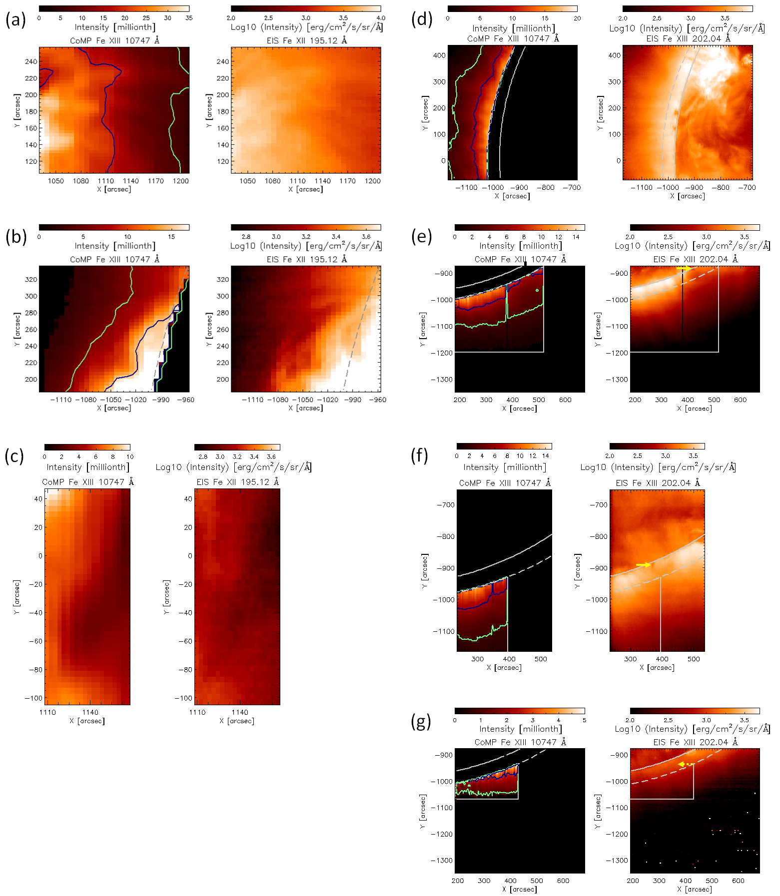
Figure 1: Raster scan CoMP and EIS intensity maps for all coronal regions. The panels show the flaring active region (a),
two quiescent active regions (b and c), an equatorial quiet region (d), two polar prominence regions (e and f), and a polar plume region (g). In each raster scan map, the Y direction shows spatial variations at a given time, while the X direction represents temporal and spatial variations. Green and blue contours show the regions where CoMP intensities are equal to 20% and 50% of their maximum intensities, respectively. In panel (c), all pixels have values higher than 20% of the maximum intensities. The gray continuous (dashed) partial circle lines indicate the solar disk (CoMP occulting disk). In panels (e-g), the yellow and yellow-dotted arrows indicate the observed prominence and polar plume, respectively. The horizontal and vertical gray lines represent the observed CoMP FOV in its pseudo raster scan. Limitations of the CoMP FOVs in solar X direction are caused by CoMP data gaps during the EIS raster scan observations. The data gaps are caused by limitations on the available time windows due to geographic and weather conditions of the ground-based CoMP observations.
By comparing LOS Doppler velocity distributions from CoMP and EIS as shown Figure 2, we find the following statistical characteristics: The CoMP and EIS Doppler velocity distributions are consistent overall in the active regions and equatorial quiet region (0.25 ≤ CC ≤ 0.7), while they are similar in the overlying loops of prominences and near the Bottom of the polar plume (0.02 ≤ CC ≤ 0.18). The differences of the Doppler velocities are within the EIS measurement accuracy in most coronal regions (≥ 87% of all pixels) except for the polar plume region (45% of pixels). These results show that CoMP observations with three-wavelength data provide reliable 2-D LOS Doppler velocity distributions in active regions and equatorial quiet region. The linear regression for the flaring active region having the highest correlation (CC = 0.7) finds a slope of 1.23, indicating that the EIS Doppler velocities are slightly larger than the CoMP ones by a factor of 1.2. When we only consider relatively bright structures whose CoMP intensities are higher than 50% of the maximum intensities, the slope is 1.5. These results, together with previous studies of the wave energy flux of propagating Alfvén wave signatures by using CoMP Doppler velocity observations (Tomczyk et al. 2007; Threlfall et al. 2013), might suggest that the wave energy flux is about 44% or 125% larger than the one obtained without the corrections found from comparison to EIS observations.
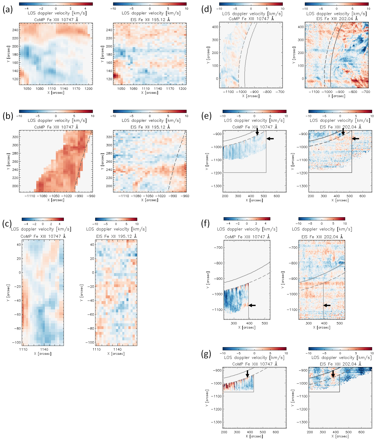
Figure 2: Raster scan CoMP and EIS Doppler maps. Each panel shows the same events as in Figure 1. We only present
CoMP Doppler velocities for locations where the CoMP intensity is higher than 20% of the maximum intensity, and EIS velocities where the EIS measurement error is below the measurement accuracy (3 km/s). In panels (e-g), black arrows indicate specific regions where the LOS Doppler velocity patterns are similar in both CoMP and EIS observations. The gray partial circle (dashed circle) and horizontal (vertical) gray lines are the same as those in Figure 1.
By comparing non-thermal line width distributions from CoMP and EIS as shown Figure 3, we find that they are similar overall in the active regions (0.06 ≤ CC ≤ 0.61), while they seem to be different in the others (-0.1 ≤ CC ≤ 0.00). CoMP non-thermal widths are similar to EIS ones within the EIS measurement accuracy in a quiescent active region (79% of pixels), while they do not match in the others (≤ 61% of pixels). The CoMP line widths are 20-40% smaller than the EIS widths. Our results indicate that although CoMP observations tend to underestimate line widths by about 30%, they might provide non-thermal width distributions in active regions. When examining the linear regression for the flaring active region having the highest correlation (CC = 0.61), the slope is 5.7, indicating that the EIS non-thermal widths are six times larger than the CoMP ones. This trend is caused by the limited non-thermal width range (15.2-21.2 km/s) in CoMP observations compared to the EIS ones (5.1-57.1 km/s). The differences in non-thermal widths between CoMP and EIS and the limited CoMP non-thermal width range are mainly caused by the limited spectral window (3.6 Å) for CoMP observations that use the three-wavelength filters. If we use five-wavelength filter CoMP observations of Fe XIII 10747 Å with a wide spectral window of 10 Å as shown in Figure 5 of Tomczyk et al. (2008), the differences might be reduced and the limited non-thermal width range might be broader. We cannot rule out the possibility that using the EIS Fe XIII 202.04 Å line instead of Fe xii 195.12 Å for comparing non-thermal widths in active regions reduces the differences; the thermal width of Fe XIII is about 11% larger than that of Fe XII, which reduces the observed non-thermal widths in EIS observations. For example, comparing the average of non-thermal widths between Fe XII and Fe XIII for four events (equatorial quiet region, two polar prominence regions, and polar plume region), we find that the non-thermal widths of Fe XIII are about 11% in average (with a range of 2-21%) smaller than those of Fe XII.
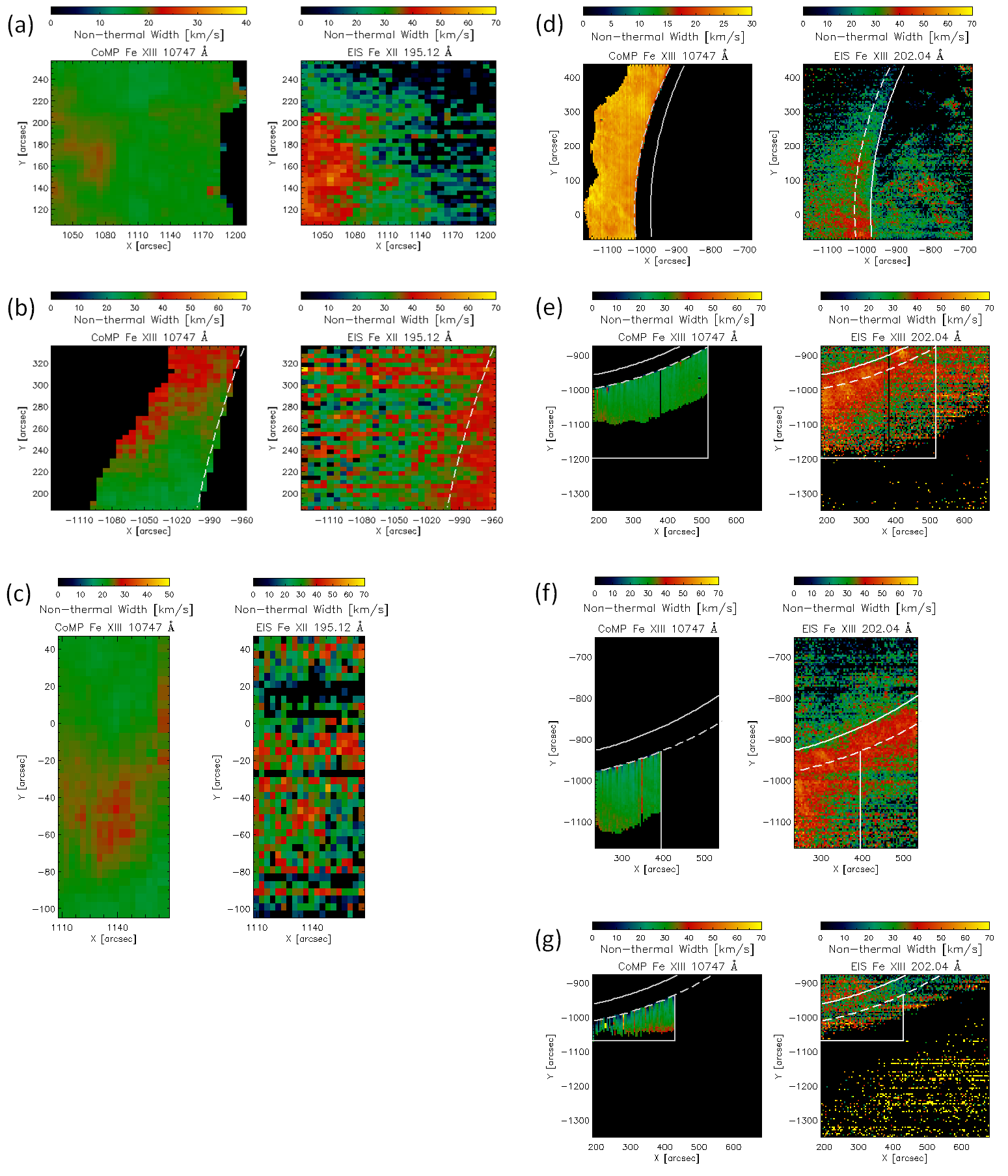
Figure 3: Raster scan CoMP and EIS non-thermal width maps. We only present CoMP non-thermal widths where CoMP intensities are higher than 20% of the maximum intensity, and EIS non-thermal widths where its measurement error is within the measurement accuracy (9 km/s) and its line width is larger than the sum of thermal and instrumental widths. The gray partial circle (dashed circle) and horizontal (vertical) gray lines are the same as those in Figure 1.
By careful investigating the non-thermal width maps for the active regions, we find that the CoMP and EIS non-thermal width distributions are similar overall while showing different trends: CoMP and EIS non-thermal widths of bright structures near the solar limb are larger than those in the faint structures far from the solar limb in the flaring active region, and they are smaller than those in the faint structures in the quiescent active regions. The non-thermal width distribution in the flaring active region might be related to Alfvén wave damping under the assumption that non-thermal plasma motions are mainly caused by the Alfvén waves. We cannot rule out the possibility that Gaussian fitting errors that occur when determining line widths on maps with small intensity-to-background ratio lead to significant changes in computed non-thermal widths as shown in Figure 10 of Brooks & Warren (2016). The non-thermal width distributions in quiescent active regions might be connected to propagating coronal Alfvén waves (Banerjee et al. 1998; Wilhelm et al. 2004; Banerjee et al. 2009) or caused by the Gaussian behavior of fits of line widths in low-intensity regions which results in larger full width at half maximum values than in high-intensity regions for given spectral lines.
Our results demonstrate that CoMP observations can provide reliable 2-D LOS Doppler velocity distributions in active regions and might provide their non-thermal width distributions. By comparing electron densities on coronal loops within a complex of active regions (AR 12579, 12582, and 12583) obtained from CoMP and Hinode/EIS data, Dudík et al. (2021) showed that CoMP observations can provide trustworthy 2-D electron density distributions in active regions. Therefore, CoMP with SDO/AIA observations can be used to detect propagating Alfvén wave signatures on different active regions at the same time, and estimate their origins, dissipation, and energy fluxes. According to the theoretical description of Alfvén-wave turbulence
heating (Chandran & Hollweg 2009; Chandran et al. 2011), the efficiency of turbulent heating depends not
only on the observed non-thermal width but also on the plasma environment such as the local Alfvén speed and
the plasma beta, which is the ratio of plasma pressure to magnetic pressure. Thus, remote-sensing observations
might be useful when investigating the turbulent heating rates for different coronal regions, and furthermore, give a better understanding of coronal heating and solar wind acceleration by Alfvén waves.
For more details, see Lee et al., Journal of the Korean Astronomical Society 54: 49 ~ 60, 2021:
Comparisons of LOS Doppler velocity and non-thermal line widths in the off-limb solar corona measured simultaneously by CoMP and Hinode/EIS.
References
1. Banerjee, D., Teriaca, L., Doyle, J. G., et al. 1998, Broadening of Si VIII Lines Observed in the Solar Polar Coronal Holes, A&A, 339, 208.
2. Banerjee, D., Perez-Suarez, D., & Doyle, J. G., 2009, Signatures of Alfvén Waves in the Polar Coronal Holes as Seen by EIS/Hinode, A&A, 501, L15.
3. Brooks, D. H., & Warren, H. P. 2016, Measurements of Non-Thermal Line Widths in Solar Active Regions, ApJ, 820, 63.
4. Culhane, J. L., Harra, L. K., James, A. M., et al. 2007, The EUV Imaging Spectrometer for Hinode, Sol. Phys., 243, 19.
5. Dudík, J., Zanna, G. D., Ryb_ak, J., et al. 2021, Electron Densities in the Solar Corona Measured Simultaneously in the Extreme Ultraviolet and Infrared, ApJ, 906, 118.
6. Chandran, B. D. G., & Hollweg, J. V., 2009, Alfvén Wave Reection and Turbulent Heating in the Solar Wind from 1 Solar Radius to 1 AU: An Analytical Treatment, ApJ, 707, 1659.
7. Chandran, B. D. G., Dennis, T. J., Quataert, E., & Bale, S. D., 2011, Incorpoating Kinetic Physics into a Two-Fluid Solar-Wind Model with Temperature Anisotropy and Low-Frequency Alfvén-Wave Turbulence, ApJ, 743, 197.
8. Threlfall, J., Moortel, I. D., McIntosh, S. W. et al. 2013, First Comparison of Wave Observations from CoMP and AIA/SDO, A&A, 556, A124.
9. Tomczyk, S., Card, G. L., Darnell, T., et al. 2008, An Instrument to Measure Coronal Emission Line Polarization, Sol. Phys., 247, 411.
10. Tomczyk, S., McIntosh, S. W., Keil, S. L., et al. 2007, Alfvén Waves in the Solar Corona, Science, 317, 1192.
11. Wilhelm, K., Dwivedi, B. N., & Teriaca, L., 2004, On the Widths of the Mg X Lines near 60 nm in the Corona, A&A, 415, 1133.
Next EIS Nugget »» coming soon...
TBC
Last Revised: 27-Oct-2011
Feedback and comments: webmaster
|