Intriguing Plasma Composition Pattern in a Solar Active Region: a Result of Non-Resonant Alfven Waves?

 

Introduction
Plasma composition in active regions is highly variable, both spatially and in time, likely reflecting the variety of processes taking place throughout an active region's evolution and in different parts of the active region. The FIP bias changes throughout the lifetime of the active region and also shows significant variations on sub-active region scales. These variations could be linked to a diverse processes including magnetic activity, wave activity, heating or magnetic topology.

In addition to this spatial and temporal variation, the FIP bias of a given location can also vary depending on the elements involved in the diagnostic used to measure it (see e.g., To et al., 2021). This is particularly important when one of the diagnostics includes intermediary FIP elements (e.g. S) which were observed to show fractionation in some cases but not others. Therefore, using more than one FIP bias diagnostic enables us to better characterise the abundance pattern in a given location - but what can this tell us about the details of the fractionation process? Here, we investigate the potential of studying plasma composition patterns using multiple FIP bias diagnostics, particularly involving variations in the behaviour of S, to obtain insight into Alfven wave activity within an active region.

Observations
The analysis is focused on active region AR12665 following an episode of new flux emergence in the preexisting magnetic field environment of the region. This led to the active region being divided into two main loop populations: the new loops formed by the flux emergence and the preexisting loops that had been there before the new flux emergence began (see Figure 1). We characterise the plasma composition patterns in these two loop populations using two FIP bias diagnostics: Si X 258.38 A (low FIP, FIP = 8.25 eV) / S X 264.22 A (high FIP, FIP = 10.36 eV) and Ca XIV 193.87 A (low FIP, FIP = 6.11 eV) / Ar XIV 194.40 A (high FIP, FIP = 15.76 eV). The results are shown in Figures 2. A FIP bias proxy is estimated in every pixel using the line ratio method, and more precise FIP bias values are calculated using a DEM and density analysis in a few key locations as illustrated in Figures 2. In the emerging loops, the Si/S and Ca/Ar FIP bias values are very similar. In the preexisting loops, however, the Si/S FIP bias values are significantly lower than the Ca/Ar ones. This difference in plasma composition pattern raises the question of whether the mechanism driving the FIP effect has different characteristics in the two loop populations, so this possibility was explored further using simulations from the ponderomotive force model.

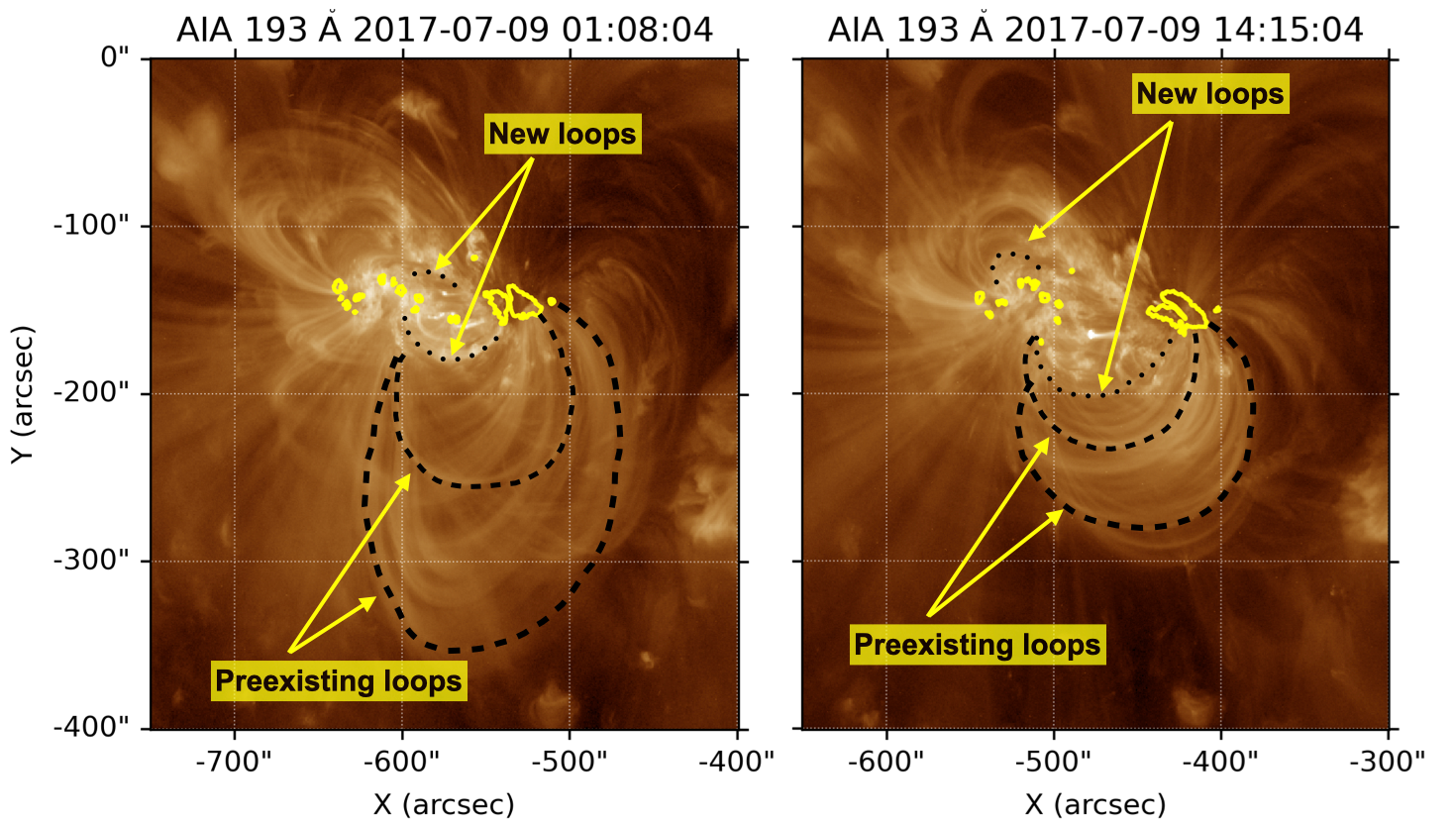
Figure 1: SDO AIA 193 A passband images at the times matching the middle time of the EIS raster scans. Yellow contours represent values below 25,000 ct/s in the continuum emission, indicating the location of the sunspots. Black dotted (dashed) lines indicate representative examples of loops belonging to the new (preexisting) loop populations.

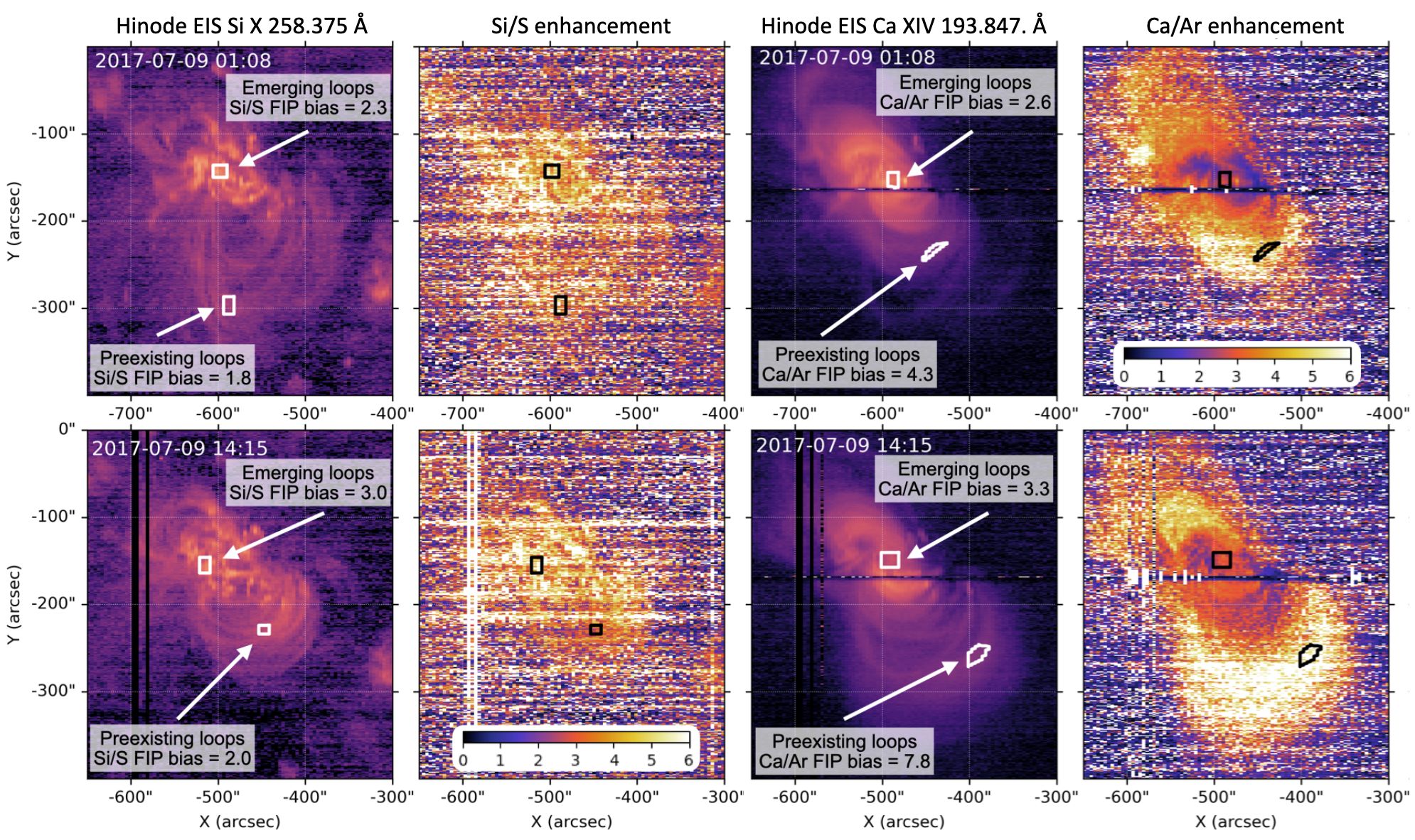
Figure 2: Hinode EIS plasma composition results. From left to right: Si X 258.38 A intensity, Si X 258.38 A/S X 264.22 A line ratio, Ca XIV 193.87 A intensity, Ca XIV 193.87 A/Ar XIV 194.40 A line ratio. The boxes indicate the locations of the macropixels used for FIP bias calculations that included a DEM analysis and density analysis.

The Ponderomotive Fractionation Model Predictions
The ponderomotive force model (Laming, 2015) is a 1D static model which proposes that the FIP effect is generated in the chromosphere by Alfven wave activity. Simulations of the ponderomotive force fractionation (see Figure 3) in loops with similar characteristics as the ones presented above suggest that the ponderomotive force driver is resonant waves in the emerging loops and non-resonant waves in the preexisting loops. This would explain the difference in plasma composition patterns observed in the two loop populations. In the resonant case, the ponderomotive acceleration is highest at the top of the chromosphere and the transition region (Figure 3e). As a result, the abundances of Si and Ca (relative to H, i.e. absolute abundances) show the highest enhancement around the top of the chromosphere and the transition region (Figure 3f). Ar and S are essentially not fractionated, so the Si/S and Ca/Ar ratios at the top of the transition region are very similar. In the non-resonant case, fractionation happens lower down in the chromosphere and is overall stronger: the ponderomotive acceleration starts increasing at the bottom of the chromosphere, reaches a maximum at the middle of the chromosphere and then decreases (Figure 3h). The abundances of Si and Ca (relative to H) start increasing from the bottom of the chromosphere, which results in stronger enhancements at the top of the transition region compared to the resonant case. Interestingly, in this case S behaves similarly to Si and Ca rather than Ar: it becomes enhanced as well, but to a lower degree than Si and Ca. As in the resonant case, Ar shows no fractionation. This could explain the strong difference between the Ca/Ar FIP bias and the Si/S FIP bias in the Hinode EIS measurements of the preexisting loops. As in the resonant case, Ca is more strongly enhanced than Si due to its higher ionization fraction. However, in the non-resonant case, the largest discrepancy between diagnostics comes from the fact that S experiences significant fractionation as well, i.e. does not behave like a high-FIP element anymore. Therefore, the enhancement of Si is underestimated when measured relative to S.

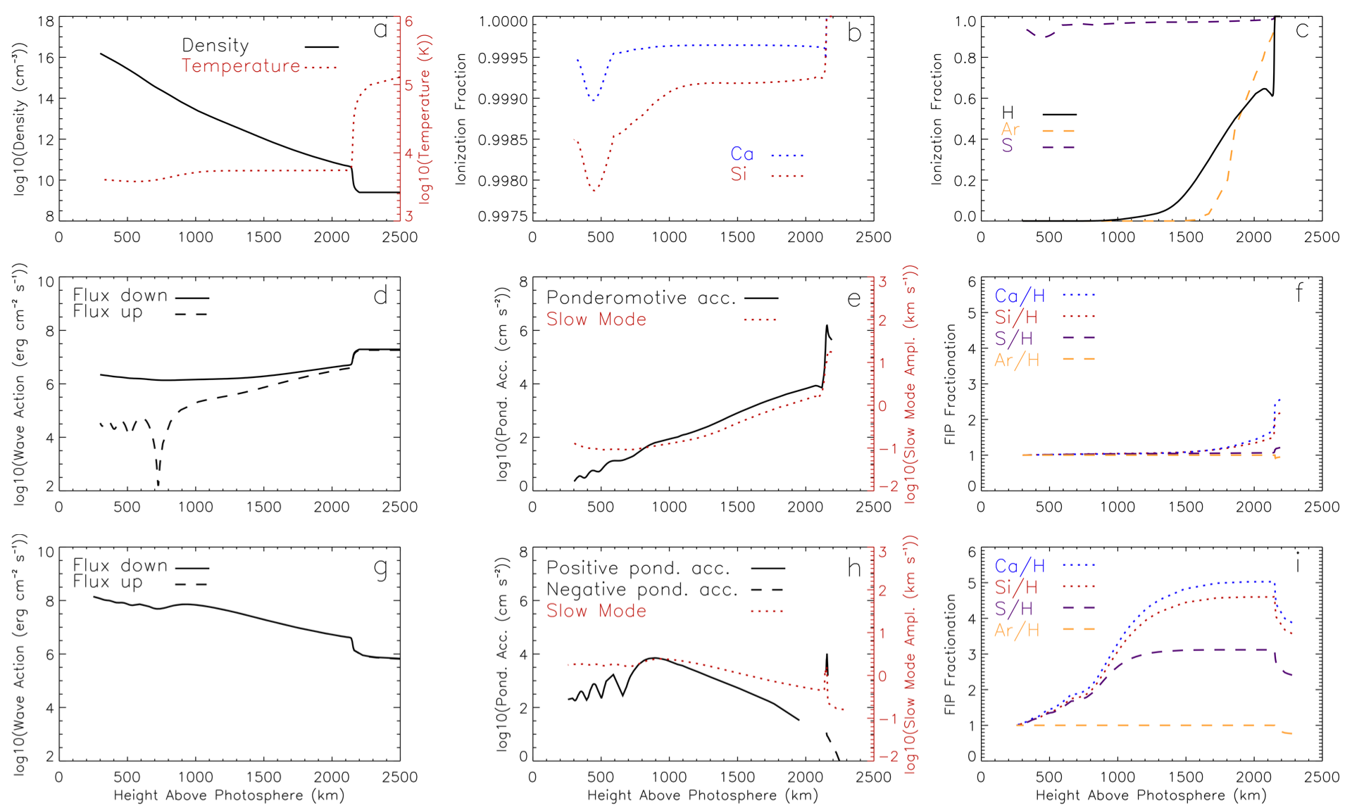
Figure 3: Ponderomotive force model predictions. First row shows the variation with height of the following parameters: a) electron temperature and density, b) ionization fraction variation for low-FIP elements, c) ionization fraction for high-FIP elements. Second row shows the variation with height of d) downward and upward Alfven wave energy fluxes for waves of assumed coronal origin e) ponderomotive acceleration f) FIP bias relative to H in the resonant fractionation case. Third row shows the variation with height of g) Alfven wave energy fluxes; the downward and upward fluxes are identical, h) ponderomotive acceleration i) FIP bias relative to H in the non-resonant fractionation case.

An interesting discussion point is the origin of these waves. In this work, we consider that the waves giving rise to the fractionation seen in the emerging loops have a coronal driver. The emerging loops make up the very active core of the active region, where nanoflares, for example, can give rise to coronal Alfven waves that are naturally at resonance with the loop. We discuss the possibility of both a coronal and a photospheric driver for the waves giving rise to the fractionation observed in the preexisting loops. The preexisting loops are less active, which means an external driver is more likely to generate the waves needed for the fractionation. The external driver could either be driven by coronal wave activity in the neighbouring loops (coronal driver) or by photospheric motions driven by the flux emergence (photospheric driver).

For more details, see:
Mihailescu et al., ApJ, 959:72, 202:
Intriguing Plasma Composition Pattern in a Solar Active Region: a Result of Non-Resonant Alfven Waves?


References
Laming, J. M. (2015). The FIP and Inverse FIP Effects in Solar and Stellar Coronae. Living Reviews in Solar Physics, 12(1):2
To, A. S. H., Long, D. M., Baker, D., Brooks, D. H., Driel-Gesztelyi, L. v., Laming, J. M., and Valori, G. (2021). The Evolution of Plasma Composition during a Solar Flare. The Astrophysical Journal, 911(2):86

 

For more details, please contact: Dr. Deb Baker.

Prev

Archive

Next

Next EIS Nugget    »»  coming soon...

TBC